Temperature, Salinity, and Stratification¶

Now that we have learned the basic thermodynamics of seawater and understood how temperature and salinity combine to determine the stratifcation of water columns, we are ready to examine the global patterns of temperature, salinity and stratification. These patterns are fascinating and reveal much about the underlying ocean circulation. We will also learn how to identify distinct water masses both in geographic space and in temperature / salinity coordinates.

import xarray as xr
from matplotlib import pyplot as plt
import hvplot.xarray
import gsw
import numpy as np
import holoviews as hv
from IPython.display import Image
hv.extension('bokeh')
plt.rcParams['figure.figsize'] = (12,7)

3D Temperature¶

def map_section_plot(data, label, data_range, levels, cmap='viridis'):
    ds = hv.Dataset(data)
    img = ds.to(hv.Image, ['lon', 'lat'], label=label)
    img = img.redim.range(**{data.name: data_range})

    posx = hv.streams.PointerX()
    vline = hv.DynamicMap(lambda x: hv.VLine(x or 180.5), streams=[posx])

    lats = np.arange(-90, 91)
    def cross_section(x):
        mesh = hv.QuadMesh((lats, woa.depth, data.sel(lon=x if x else 180, method='nearest').data[:-1]),
                           kdims=['lat', 'depth'], label=(label + ' Section'))
        contours = hv.operation.contours(mesh, levels=levels,
                                         overlaid=False, filled=True)
        return contours

    
    crosssection = hv.DynamicMap(cross_section, streams=[posx])
    layout = (img * vline) + crosssection 
    
    # set view options
    dict_spec = {'Image': {'plot': dict(colorbar=True, toolbar='above', width=600),
                           'style': dict(cmap=cmap)},
                 'NdOverlay': {'plot': dict(bgcolor='grey', invert_yaxis=True, width=600, height=200)},
                 'Layout': {'plot': dict(show_title=False)},
                 'Polygons': {'plot': dict(colorbar=True, invert_yaxis=True, width=600),
                              'style': dict(cmap=cmap, line_width=0.1)}
                 }
    layout.cols(1)
    layout = layout.opts(dict_spec)   
    return layout

map_section_plot(woa.t_an, 'Temperature', (-2,30), np.arange(-2,31), cmap='RdBu_r')

Observations¶

The warmest water is near the surface in the tropical regions, forming a bowl-shaped lens in the upper ~800 meters. This is called the thermocline.
There are clear zonal asymmetries in surface temperature. The western boundaries of the basins tend to be warmer, with colder water near the eastern boundaries.
There is something special going on at the equator, especially in the Pacific. It’s relatively cold, and the thermocline is shallow.
Below 1000 m, the water is mostly very cold (< 5 C).
In the polar regions, the coldest water is actually found near the surface! There is a mid-depth temperature maximum.

3D Salinity¶

map_section_plot(woa.s_an, 'Salinity', (32,38), np.arange(32,38.1, 0.25))

Observations¶

Salinity has a more complex structure than temperature.
The Atlantic is overall saltier than the Pacific.
The saltiest parts of the oceans are the extra-tropical-latitudes.
The equator is relatively fresh near the surface.
Salinity sections across the Atlantic reveal the interleaving of several different water masses including
- Mediterranean Water
- North Atlantic Deep Water
- Antarctic Intermediate Water
- Antarctic Bottom Water

3D Potential Density¶

map_section_plot(woa.sigma_0, 'Potential Density (sigma0)', (22.,28.), np.arange(22,28.1, 0.25))

map_section_plot(woa.sigma_4, 'Potential Density (sigma4)', (40.,46.5), np.arange(40,46.5, 0.25))

Observations¶

Potential density reflects the mechanical stratification of the ocean most closely of any of the quantities we have examined so far.

For the most part, potential density is monotonically increasing with depth.
BUT there are exceptions. Each potential density variable shows density “inversions” far from its reference level.
Potential density surface approximately represent pathways that water parcels can move along without experiencing a restoring force. Therefore, they serve as connections between the surface and deep ocean.
These connections are strongest in the Southern Ocean region.

Image('02_images/neutral_plane.png')

_images/02-c_ocean_temperature_salinity_stratification_23_0.png

woa['thick'] = woa.depth.diff(dim='depth')
woa['thick'][0] = 5
# add an area element
earth_radius =  6.371e6
tot_area = (4 * np.pi * earth_radius**2)
woa['area'] = earth_radius**2 * np.radians(1.) * np.radians(1.) * np.cos(np.radians(woa.lat))
woa['vol'] = woa.thick * woa.area
vol_full, _ = xr.broadcast(woa.vol, woa.lon)

fig, (ax1, ax2) = plt.subplots(2)

ax1.hist(woa.c_t.where(woa.c_t).values.ravel(), bins=100, density=True, range=(-2,30),
         weights=vol_full.where(woa.c_t).values.ravel());
ax2.hist(woa.s_a.where(woa.c_t).values.ravel(), bins=100, density=True, range=(32,38),
         weights=vol_full.where(woa.s_a).values.ravel());
ax1.set_xlabel(r'Temperature ($^\circ$C)')
ax2.set_xlabel("Salinity (g / kg)")
plt.tight_layout()
plt.close()

Temperature and Salinity Probability Distributions¶

fig

_images/02-c_ocean_temperature_salinity_stratification_27_0.png

from matplotlib.colors import LogNorm
fig, ax = plt.subplots()
hb = ax.hexbin(woa.s_an.values.ravel(), woa.c_t.values.ravel(),
           C=vol_full.values.ravel(), reduce_C_function=np.sum,
           extent=(30,40,-3,30), gridsize=50, bins='log',
           cmap='RdYlBu_r')
plt.colorbar(hb)
ax.set_ylabel(r'Temperature ($^\circ$C)')
ax.set_xlabel("Salinity (g / kg)")
plt.close()

Joint T/S Distribution¶

fig

_images/02-c_ocean_temperature_salinity_stratification_30_0.png

#pal = seaborn.palettes.color_palette(n_colors=len(basins_main))
fig, ax = plt.subplots()
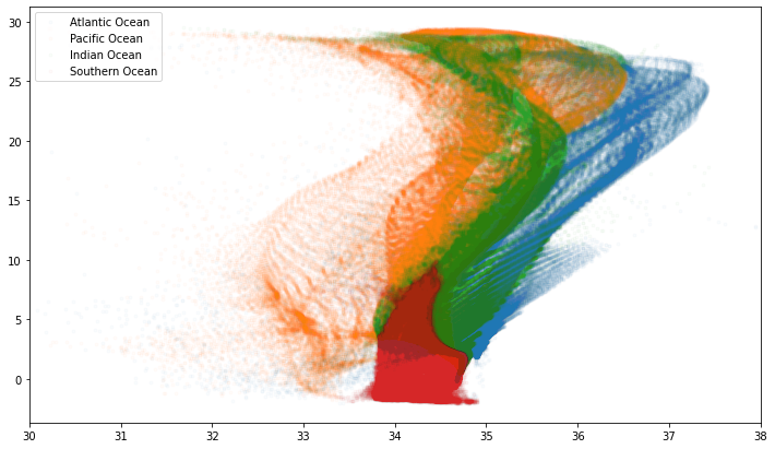
for (bnum, bname) in basins_main.items():
    ax.plot(
        woa.s_an.where(woa.basin==bnum).values.ravel(),
        woa.c_t.where(woa.basin==bnum).values.ravel(),
        '.',  alpha=0.02, label=bname
    )
ax.set_xlim(30,38)
ax.legend(loc='upper left', frameon=True)
plt.close()
# blue green red purple

T/S Distribution by Basin¶

fig

_images/02-c_ocean_temperature_salinity_stratification_33_0.png

Ocean Warming¶

We have been looking at climatologies. But we can’t forget that the ocean is warming!

Data from https://www.nodc.noaa.gov/OC5/3M_HEAT_CONTENT/.

fig

_images/02-c_ocean_temperature_salinity_stratification_38_0.png

Intro to Physical Oceanography

Temperature, Salinity, and Stratification¶

Data Source: World Ocean Atlas¶

3D Temperature¶

Observations¶

3D Salinity¶

Observations¶

3D Potential Density¶

Observations¶

Temperature and Salinity Probability Distributions¶

Joint T/S Distribution¶

T/S Distribution by Basin¶

Thermohaline Circulation¶

Ocean Warming¶