Thermodynamics of Seawater¶

import xarray as xr
from matplotlib import pyplot as plt
import numpy as np
import gsw
%matplotlib inline
plt.rcParams['figure.figsize'] = (12,7)
from IPython.display import SVG, display, Image, display_svg
import holoviews as hv
hv.extension('bokeh')

TEOS-10: The Official Reference¶

TEOS-10 = Thermodynamic Equation Of Seawater - 2010

TEOS-10 is based on a Gibbs function formulation from which all thermodynamic properties of seawater (density, enthalpy, entropy sound speed, etc.) can be derived in a thermodynamically consistent manner. TEOS-10 was adopted by the Intergovernmental Oceanographic Commission at its 25th Assembly in June 2009.

The thermodynamic properties of seawater are determined experimentally in a laboratory!

TEOS-10 Website and Manual ¶

TEOS-10 Software:

What is Seawater?¶

seawater molecule

Model of hydrogen bonds between molecules of water.

Attribution: By User Qwerter at Czech wikipedia: Qwerter. Transferred from cs.wikipedia; Transfer was stated to be made by User:sevela.p. Translated to english by by Michal Maňas (User:snek01). Vectorized by Magasjukur2. License: CC BY-SA 3.0. Via Wikimedia Commons.

Water Chemistry¶

Water is a polar molecule with a strong dipole moment. This means that there can be strong intermolecular electric forces, as hydrongen atoms of one molecule attract the oxygen atom of another. This chemical property is ultimately responsible for many of water’s exceptional physical properties such as:

Very high surface tension
Very high heat capacity
Very high latent heat of fusion
Very high latent heat of evaporation

The last three properties in particular have major consequences for Earth’s climate.

Phases of Water¶

Phase diagram of water as a log-lin chart with pressure from 1 Pa to 1 TPa and temperature from 0 K to 650 K. Simplified version.

Attribution: By author of the original work: Cmglee (Own work) License:CC BY-SA 3.0]. Via Wikimedia Commons

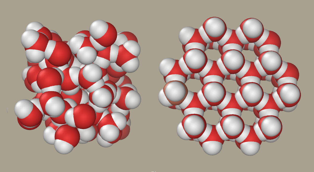
Liquid water and ice molecular structure.

Attribution: By P99am (Own work). License: CC BY-SA 3.0. Via Wikimedia Commons

Salinity¶

Graphic breakdown of water salinity, defining freshwater, brackish water, saltwater, and brine water.

Attribution: By Peter Summerlin (Own work). License: CC BY-SA 3.0. Via Wikimedia Commons

Seawater Composition¶

Proportion of salt to sea water (right) and chemical composition of sea salt

Attribution: By Hannes Grobe, Alfred Wegener Institute for Polar and Marine Research, Bremerhaven, Germany; SVG version by Stefan Majewsky (Own work). Licesnse: CC BY-SA 2.5. Via Wikimedia Commons

How do we describe and measure salinity?¶

Absolute Salinity ($S_A$) represents, to the best available accuracy (and with certain caveats), the mass fraction of dissolved solute in so-called Standard Seawater with the same density as that of the sample. $S_A$ is the quantity used in the latest seawater equation of state, TEOS-10. $S_A$ has units of g / kg, i.e. mass fraction parts per thousand.

$S_A$ is not measured directly. In practice, salinity is inferred from the conductivity of seawater (which can be measured in-situ with electronic instruments) and reported as “practical salinity” $S_P$. The $S_P$ measurements are then converted to $S_A$ based on either measurements of other trace chemicals or estimated based on the geographic location of the sample. Most archived data is reported in $S_P$, not $S_A$. TEOS-10 is a new standard that is slowly being adopted by the community.

CTD¶

Parts of a CTD (Conductivity, Temperature, Depth), disassembled. Oceanographic device to determine water masses in the oceans from research vessels: - electronics with sensors for conductivity, temperature and pressure (Manufactured by ME GRISARD GMBH in the 1980s) - cage to protect sensors - water tight conectors - housing for high water pressure

By Hannes Grobe (Own work) [CC BY 3.0 (http://creativecommons.org/licenses/by/3.0)], via Wikimedia Commons

Pressure¶

Pressure is an isotropic “force per square meter”

Pressure has units of “Pascals”.

\[ Pa = \frac{N}{m^2} = \frac{kg}{m s^2} \]

“Sea pressure” $p$ is absolute pressure minus a constant reference atmospheric pressure:

\[ p = P - P_0 \]

where $P_0 = 101,325$ Pa. In oceanography we use decibars (dbar) as units.

\[ 1 dbar = 10^5 Pa \]

Question: Approximately how many dbar of pressure are needed to equal $P_0$?

Hydrostatic Balance¶

How much pressure does the water column exert? In other words, what is the weight of 1 square meter of ocean?

\[ p(z) = g \int_z^0 \rho(z') dz' \]

The pressure at depth $z$ is given by the mass of water above. We can re-express this as

\[ \boxed{\frac{\partial p}{\partial z} = - g \rho} \]

This equation is known as the hydrostatic balance.

z = np.arange(0, -5000, -1)
z_eq = xr.DataArray(z, dims=['p'], coords={'p': gsw.p_from_z(z, lat=0)}, name='z')
z_hi = xr.DataArray(z, dims=['p'], coords={'p': gsw.p_from_z(z, lat=70)}, name='z')
z_eq.sel(p=1008, method='nearest')

<xarray.DataArray 'z' ()>
array(-1000)
Coordinates:
    p        float64 1.008e+03

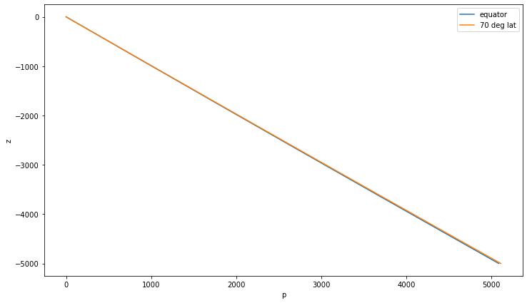
Approximate Hydrostatic Balance¶

Just use the “average” density $$ p(z) = g \int_z^0 \overline{\rho}(z') dz' $$

–> pressure is only a function of depth (and gravity)

Pressure at 1000 m depth: 1008 dbar

z_eq.plot(label='equator'); z_hi.plot(label='70 deg lat'); plt.legend()

<matplotlib.legend.Legend at 0x7f05a8252730>

_images/02-a_thermodynamics_of_seawater_19_1.png

Temperature and Heat Content¶

In general, the thermal energy of a material is given by

\[ U = \int \int \int \rho c_p T dv \]

where $\rho$ is the density, $c_p$ is the heat capacity, and $T$ is the temperature. The units of energy are Joules

Let’s compare the heat that can be stored by the ocean and the atmosphere. The following table gives values for air and seawater near sea level.

Parameter	$\rho$ (kg m$^{-3}$)	$c_p$ (J K$^{-1}$ kg$^{-1}$)
Atmosphere	1.3	1004
Ocean	1023	4218

Question: How much more heat can be stored in 1 square meter of ocean than one square meter of air?

Internal Energy¶

Temperature $T$ is not conserved under adiabatic displacements or addition / subtraction of salinity.

t0 = 10                        # initial temperature, degrees C
p0 = 0                         # initial pressure, dbar
sa0 = 35                       # initial absolute salinity
ct0 = gsw.CT_from_t(sa0,t0,p0) # calculate intial conservative temperature
p = 4000                       # new pressure
t1 = gsw.t_from_CT(sa0,ct0,p)  # new temperature

print(f'Initial temp: {t0:.3f}, conservative temp: {ct0:.3f}')
print(f'Final   temp: {t1:.3f}, conservative temp: {ct0:.3f}')

Initial temp: 10.000, conservative temp: 9.993
Final   temp: 10.562, conservative temp: 9.993

def change_in_temperature(initial_sa, initial_t, initial_p):
    ct0 = gsw.CT_from_t(initial_sa, initial_t, initial_p)
    # this is conserved
    
    # plotting parameters
    sa_min, sa_max = 30, 40
    p_min, p_max = 0, 6000
    sa_range = np.linspace(sa_min, sa_max, 100)
    p_range = np.linspace(p_min, p_max, 80)
    t = gsw.t_from_CT(sa_range[np.newaxis], ct0, p_range[:,np.newaxis])
    delta_t = t - initial_t
    #t = sa_range[np.newaxis] *  p_range[:,np.newaxis]
    # make into an xarray dataarray
    da = xr.DataArray(delta_t, dims=['P', 'S_A'],
                      coords={'S_A': sa_range, 'P': p_range})
    
    #bounds = (sa_min, p_min, sa_max, p_max)   # Coordinate system: (left, bottom, top, right)
    img = hv.Image(da, label="Temperature Change")
    delta_t_range = (-1.5, 1.5)
    img = img.redim.range(z=delta_t_range)
    
    levels = np.arange(*(delta_t_range + (0.1,) )) 
    contours = hv.operation.contours(img, levels=levels, overlaid=False, filled=True)
    return contours

%%opts Polygons [width=500 height=400 colorbar=True tools=['hover'] toolbar=None] (cmap='RdBu_r')
hv.HoloMap({t: change_in_temperature(35, t, 0) for t in range(0, 20)}, kdims=['initial temp'])

Enthalpy and Conservative Temperature¶

Specific enthalpy is represented by $h$ and has units of J/kg. A change in $h$ is equal to the change in the internal energy of the system (thermal and chemical), plus the pressure work that the system does on its surroundings (compressibility), at constant pressure.

Potential enthalpy $h_0$ is the enthalpy a water parcel would have if brought adiabatically to surface pressure.

The conservative temperature is defined in TEOS-10 as

\[ \Theta = \frac{h_0}{c_p^0} \]

where $c_p^0$ is a constant scale factor. The value of $c_p^0$ is 3991.868 J kg$^{-1}$ K$^{-1}$.

A more complete measure of heat content of the ocean is

\[ \iiint \rho h_0 dv = c_p^0 \iiint \rho \Theta dv \]

This change in this quantity is proportional to the heat flux through the ocean surface. Furthermore $\Theta$ is conserved following the fluid flow. (More on this to come.)

Prior to TEOS-10, potential temperature ($\theta$) was the preferred temperature variable. $\theta$ is the temperature that the water would have if it were brought adiabatically to the surface. Potential temperature was abandonded because it is not a conserved quantity and is not proportional to the heat content of the fluid.

t0 = 10.                      # initial conservative temperature, degrees C
p0 = 2000                     # initial pressure
sa0 = 38.                     # initial absolute salinity
ct = gsw.CT_from_t(sa0,t0,p0) # conservative temperature
tp = gsw.pt_from_CT(sa0,ct)   # potential temperature

print(ct, tp)

9.677429919404045 9.739419202041663

Density¶

The density $\rho$ is an extremely important quantity. Density has units kg m$^{-3}$ and represents the amount of mass per unit volume.

Density is a nonlinear function of $S_A$, $\Theta$, and $p$.

def density(p):    
    # plotting parameters
    sa_min, sa_max = 30, 40
    p_min, p_max = 0, 6000
    sa_range = np.linspace(sa_min, sa_max, 100)
    ct_range = np.linspace(-2, 35, 120)
    rho = gsw.rho(sa_range[np.newaxis], ct_range[:,np.newaxis], p)
    da = xr.DataArray(rho, dims=['T_C', 'S_A'], name='Density',
                      coords={'S_A': sa_range, 'T_C': ct_range})
    
    img = hv.Image(da, label="Density")
    levels = np.arange(10,60) + 1000
    contours = hv.operation.contours(img, levels=levels, filled=True, overlaid=False)
    return contours

%%opts Polygons [width=500 height=400 colorbar=True tools=['hover'] toolbar=None] (cmap='viridis')
hv.HoloMap({p: density(p) for p in range(0, 5001, 1000)}, kdims=['pressure'])

Question: What is the impact of $S_A$, $\Theta$ and $p$ on density?

Thermal Expansion¶

When water warms, it expands, and its density goes down. We measure thermal expansion as the relative change in density with respect to consevative temperature when pressure and salinity are held fixed:

\[ \alpha^\Theta = \alpha^\Theta(S_A, \Theta, p) = -\frac{1}{\rho} \frac{\partial \rho}{\partial \Theta}|_{S_A, p} \]

The minus sign is a convention to make $\alpha^\Theta$ positive.

Question: What are the units of $\alpha^\Theta$?

def thermal_expansion(p):    
    # plotting parameters
    sa_min, sa_max = 30, 40
    p_min, p_max = 0, 6000
    sa_range = np.linspace(sa_min, sa_max, 100)
    ct_range = np.linspace(-2, 35, 120)
    alpha = gsw.alpha(sa_range[np.newaxis], ct_range[:,np.newaxis], p)
    da = xr.DataArray(alpha, dims=['T_C', 'S_A'], name='alpha',
                      coords={'S_A': sa_range, 'T_C': ct_range})
    
    img = hv.Image(da, label="Thermal Expansion Coefficient")
    levels = np.arange(0,60,5)*1e-5
    contours = hv.operation.contours(img, levels=levels, overlaid=False, filled=True)
    return contours

# help with formatting
# http://bokeh.pydata.org/en/latest/docs/reference/models/formatters.html#bokeh.models.formatters.TickFormatter
from bokeh.models.formatters import PrintfTickFormatter
tf = PrintfTickFormatter(format='%3.2e')

%%opts Polygons [width=500 height=400 colorbar_opts={'padding': 10, 'formatter': tf, 'label_standoff': 12} colorbar=True tools=['hover'] toolbar=None] (cmap='Greens')
hv.HoloMap({p: thermal_expansion(p) for p in range(0, 5001, 1000)}, kdims=['pressure'])

Haline Contraction¶

When water gains salt, its density goes up. We measure this with the haline contraction coefficient $\beta^\Theta$.

\[ \beta^\Theta = \beta^\Theta(S_A, \Theta, p) = \frac{1}{\rho} \frac{\partial \rho}{\partial S_A}|_{\Theta, p} \]

def haline_contraction(p):    
    # plotting parameters
    sa_min, sa_max = 30, 40
    p_min, p_max = 0, 6000
    sa_range = np.linspace(sa_min, sa_max, 100)
    ct_range = np.linspace(-2, 35, 120)
    beta = gsw.beta(sa_range[np.newaxis], ct_range[:,np.newaxis], p)
    da = xr.DataArray(beta, dims=['T_C', 'S_A'], name='beta',
                      coords={'S_A': sa_range, 'T_C': ct_range})
    
    img = hv.Image(da, label="Haline Contraction Coefficient")
    levels = np.arange(65,80)*1e-5
    contours = hv.operation.contours(img, levels=levels, overlaid=False, filled=True)
    return contours

%%opts Polygons [width=500 height=400 colorbar_opts={'padding': 10, 'formatter': tf, 'label_standoff': 12} colorbar=True tools=['hover'] toolbar=None] (cmap='Purples')
hv.HoloMap({p: haline_contraction(p) for p in range(0, 5001, 1000)}, kdims=['pressure'])

Adiabatic Compressibility¶

When conservative temperature and absolute salinity are held fixed as pressure is increased, the fluid is compressed. This property is quantified by the compressibility coefficient

\[ \kappa = \frac{1}{\rho}\frac{\partial \rho}{\partial p}|_{S_A, \Theta} \]

The speed of sound $c$ in seawater is directly related to compressibility.

\[ c = \frac{1}{\sqrt{\rho \kappa}} \]

def compressibility(p):    
    # plotting parameters
    sa_min, sa_max = 30, 40
    p_min, p_max = 0, 6000
    sa_range = np.linspace(sa_min, sa_max, 100)
    ct_range = np.linspace(-2, 35, 120)
    c = gsw.sound_speed(sa_range[np.newaxis], ct_range[:,np.newaxis], p)
    da = xr.DataArray(c, dims=['T_C', 'S_A'], name='c',
                      coords={'S_A': sa_range, 'T_C': ct_range})
    
    img = hv.Image(da, label="Sound Speed")
    levels = np.arange(140,180,2)*10
    contours = hv.operation.contours(img, levels=levels, overlaid=False, filled=True)
    return contours

%%opts Polygons [width=500 height=400 colorbar_opts={'padding': 10, 'formatter': tf, 'label_standoff': 12} colorbar=True tools=['hover'] toolbar=None] (cmap='Blues')
hv.HoloMap({p: compressibility(p) for p in range(0, 5001, 1000)}, kdims=['pressure'])

An Approximate Equation of State¶

This equation contains the “essential” nonlinearities in the equation of state of seawater.

\[ \rho \simeq \rho_0 \left [ 1 - \frac{gz}{c_0^2} - \alpha_0(1 - \gamma_B z)(\Theta - \Theta_0) - \frac{\gamma_C}{2}(\Theta - \Theta_0)^2 + \beta_0 (S_A - S_{A0} ) \right ] \]

where $\rho_0$, $c_0$, $\alpha_0$, $\gamma_B$, $\gamma_C$, and $\beta_0$ are all positive constants. Here we have assumed that pressure $p$ is simply proportional to depth $z$. (As we will see next, this is a very good approximation.)

The parameter $\gamma_B$ expresses the nonlinear effect of thermobaricity. The parameter $\gamma_C$ expresses the nonlinear effect of cabbeling.

Intro to Physical Oceanography