Ocean State Estimation
What do we want to know about the ocean?
From the point of view of climate science, some of the most important questions we want to answer about the ocean are:
What is the mean state of the ocean’s master variables (temperature, salinity, velocities, and sea-surface height)?
How does the ocean state vary in time?
What is the strength and direction of ocean transports of mass, heat, and salt; and how do these transports vary in time?
What is the exchange of heat, freshwater, and momentum with the atmosphere?
Ocean observations come from a huge range of difference sources, but for the most part, there are few direct observations of these quantities. Furthermore these observations have their own errors and inconsistencies. How can they be synthesized into a “best guess” of the true ocean state? This is a challenging scientific and engineering problem.
Ocean General Circulation Models

Ocean General Circulation Models (GCMs) encode our understanding of the laws of physics into a computer program that can be run on a computer (usually a supercomputer). They solve numerically the appropriate physical equations (usually partial differential equations; e.g. momentum equation, heat equations) subject to specified boundary conditions (e.g. the atmospheric state).
Ocean models divide the ocean up into discrete “grid cells”. The smaller the cells, the more accurate and detailed the simulation; this is called “resolution”. But high resolution is also expensive…the time it takes to solve the equations depends roughly on \(\Delta X^3\), where \(\Delta X\) is the size of the grid box (in meters).
Ocean models aren’t perfect, but they are consistent…
Ocean models do not provide a perfect representation of the ocean. But they do provide a consistent one. A well-formulated ocean model exactly conserves quantities like heat, energy, and momentum, just like the real ocean.
The butterfly effect

However, even a perfect model would not reproduce the real ocean state and its evolution over time exactly. Due to the inherent chaos in the governing equations, miniscule differences in initial conditions between the model and the real world would eventually amplify and cause the simulation to diverge from the real world. This is often called the Butterfly Effect.
Data Assimilation
Data assimilation is a set of methologies for making a simulation consistent with observations.
The state estimate uses a form of data assimilation called 4D Var or “four-dimensional variational” assimilation. This works by iteratively adjusting the initial conditions and boundary conditions of the simulation to bring it as close as possible to the observations. The observations are weighed relative to their uncertainties. This method produces estimates that are consistent with diverse observations yet still respect the conservation properties encoded in the GCM.

Image credit:
Zaron E.D. (2011) Introduction to Ocean Data Assimilation. In: Schiller A., Brassington G. (eds) Operational Oceanography in the 21st Century. Springer, Dordrecht. https://doi.org/10.1007/978-94-007-0332-2_13
ECCO: Estimating the Circulation and Climate of the Ocean
In this class, we will work with data from the NASA ECCO Ocean State Estimate. This product is the most comprehensive ocean state estimate for looking at things like ocean transport and budgets.
Let’s first review the data sources used to constrain ECCO.
Sea Surface Height
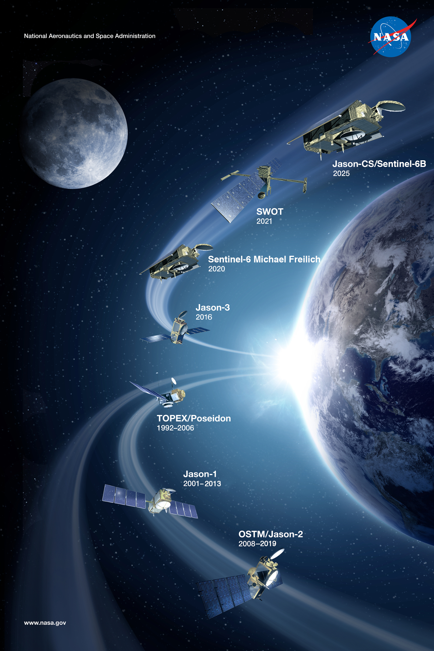
Ocean dynamic topography as measured by from space provides an important constraint on ocean heat and salt content, as well as geostrophic currents.
More info about sea level data are available from https://sealevel.jpl.nasa.gov/
Data used in ECCO include ERS-1/2 (1992-2001), TOPEX/Poseidon (1993-2005), GFO (2001-2007), ENVISAT (2002-2012), Jason-1 (2002-2008), Jason-2 (2008-2017), CryoSat-2 (2011-2017), SARAL/AltiKa (2013-2017), Jason-3 (2016-2017)
How we measure Sea Surface Height from space

Via https://commons.wikimedia.org/wiki/File:Poseidon.graphic.jpg
In Situ Temperature and Salinity

Temperature
Argo floats (1995-2017), CTDs (1992-2017), XBTs (1992-2017), marine mammals (APB 2004-2017), gliders (2003-2017), Ice-Tethered Profilers (ITP, 2004-2017), moorings (1992-2017)
Salinity
CTDs (1992-2017), moorings (1992-2017), Argo floats (1997-2017), gliders (2003-2017), marine mammals (APB 2004-2017), ITP (2004-2017)
Argo Float distribution

via https://commons.wikimedia.org/wiki/File:Argo_floats_in_Feb._2018_colour_coded_by_country.png
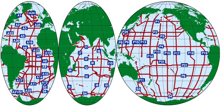
World Ocean Circulation (WOCE) & GO-Ship Hydrography
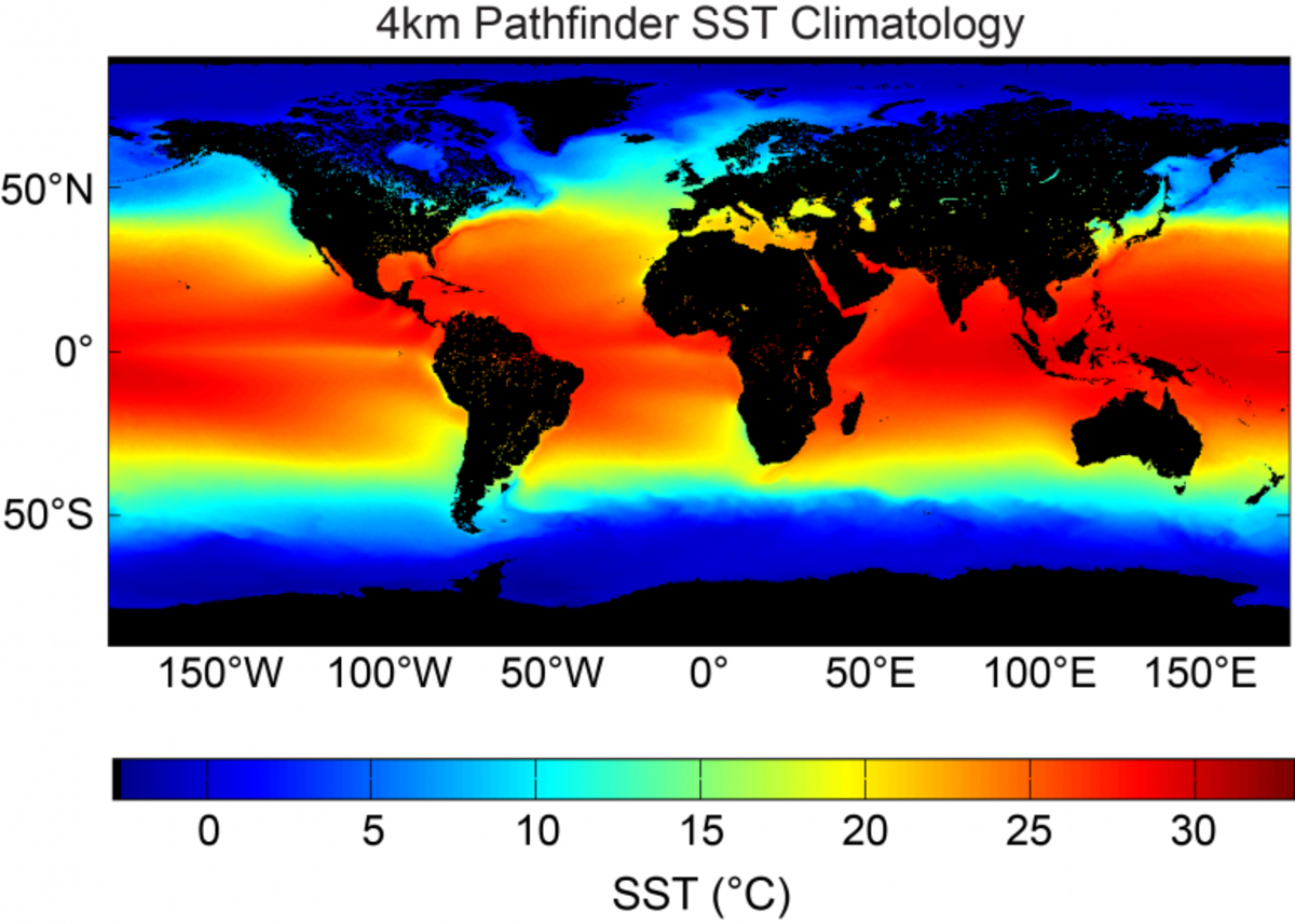
Sea Surface Temperature
From the Advanced Very High Resolution Radiometer (AVHRR)
https://www.ncei.noaa.gov/products/climate-data-records/pathfinder-sea-surface-temperature
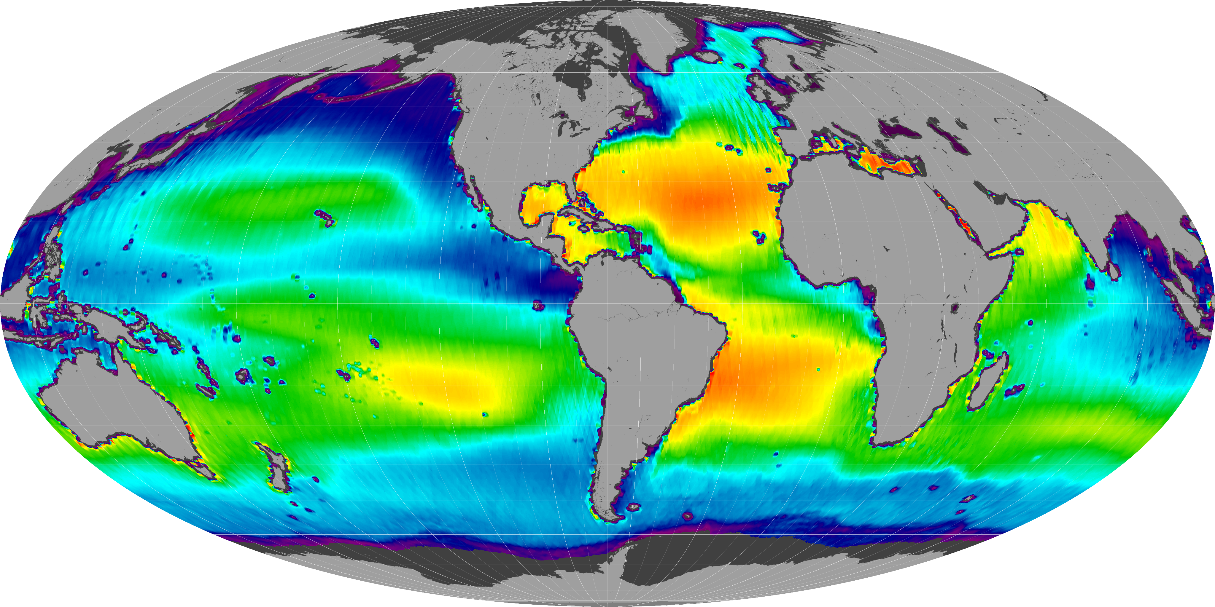
Sea Surface Salinity
NASA Aquarius mission
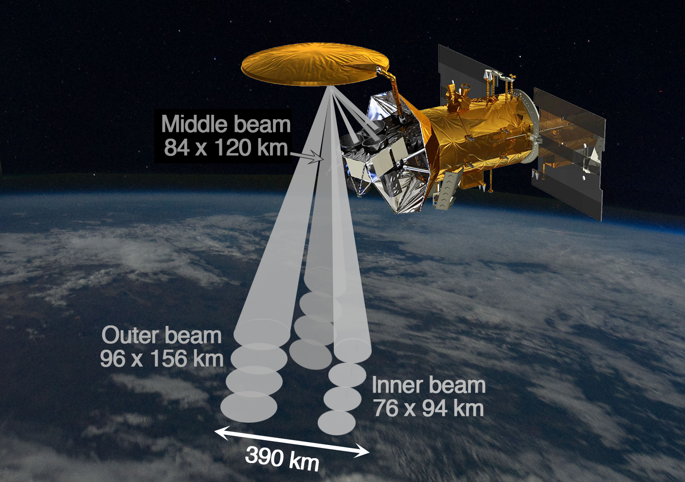
Aquarius Instrument
Aquarius was an active/passive microwave remote sensor that measured brightness temperature and radar backscatter at L-band. The antenna system’s reflector produced three beams (pointed at incidence angles 25.8°, 33.8°, and 40.3° for the inner, middle, and outer beams, respectively) to obtain measurements in a push-broom fashion from feed horns pointed perpendicular to the flight direction. The beams created three fields of view at the Earth’s surface resulting in a data swath of approximately 390km. Credit: NASA.
via https://salinity.oceansciences.org/gallery-images-more.htm?id=79
Sea Ice Concentration
Scanning Multichannel Microwave Radiometer (SMMR) instrument on the Nimbus-7 satellite
Special Sensor Microwave/Imager (SSM/I) and Special Sensor Microwave Imager/Sounder (SSMIS) and instruments on the Defense Meteorological Satellite Program’s (DMSP)

Ocean Bottom Pressure
NASA Gravity Recovery and Climate Experiment (GRACE).

Ocean Mass ↔️ Bottom Pressure
The mass of the water column at each point on the Earth’s surface is given by
and, via the hydrostatic balance, the ocean bottom pressure is just
The GRACE mission measures slight changes in Earth’s gravitational field, which are due to fluctuations in ocean mass.