\( \newcommand{\pd}[2]{ \frac{\partial #1}{\partial #2} } \newcommand{\od}[2]{\frac{d #1}{d #2}} \newcommand{\td}[2]{\frac{D #1}{D #2}} \newcommand{\ab}[1]{\langle #1 \rangle} \newcommand{\bss}[1]{\textsf{\textbf{#1}}} \newcommand{\ol}{\overline} \newcommand{\olx}[1]{\overline{#1}^x} \)
Southern Ocean Circulation
Basic Setup
We will use the Boussinesq momentum equations to describe a simple model for the southern ocean circulation. For simplicity, we will use Cartesian coordinates. We will be focused particularly on the zonal momentum balance, which reads
where \(\tau_x\) is the zonal component of the frictional stress. For completeness, we also note the incompressibility equation
hydrostatic balance
and the buoyancy equation
Where \(B\) is the vertical turbulent buoyancy flux.
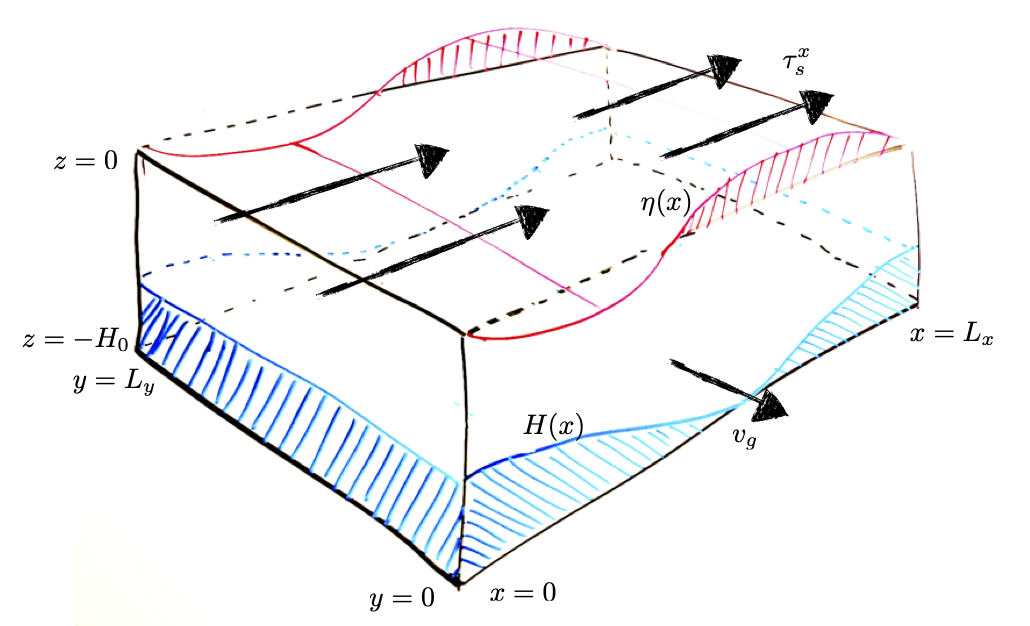
Fig. 1 Cartoon showing the domain of the idealized ACC problem.
Zonal Momentum Balance in a Barotropic Model
If we assume the density is constant (\(b=0\)), then the hydrostatic balance tells us that pressure doesn’t vary with depth. This situation is called barotropic: “baro” means pressure and “tropic” means constant. Pressure gradients can come only from the free surface \(\eta\): \(\phi = g \eta\).
Now consider an integral over the full depth of the water column and across a closed circumpolar path in the \(x\) direction. (For simplicity, we assume this path is a latitude circle, but the results generalize to any circumpolar contour.) Assuming a steady state, we find
where \(\tau^x_s\) is the frictional stress at the surface and \(\tau^x_b\) is the frictional stress at the bottom. Mass conservations requires that the term on the left-hand side vanish; otherwise mass would be flowing into or out of the Southern Ocean. The first term on the right-hand side is a Reynolds stress; this is generally negligible on the planetary scale, and we will neglect it from here on. However, it may play an important role on smaller scales, such as within the multiple jets of the ACC.
A key question is whether the bottom is flat (\(H = const\)) or rather depends on \(x\) (\(H = H(x)\)). Application of Leibnitz rule allows us to simplify the pressure term into
where \(\phi_s\) is the surface pressure and \(\phi_b\) is the bottom pressure. The first term cancels exactly via the fundamental theorem of calculus, since the integral is around a closed path. The second term cancels approximately because the surface pressure (the atmospheric load) is negligible. We are left with only the final term, the topographic form stress.
We can simplify our notation a lot by defining a zonal average, i.e.
which allows us to write the vertically and zonally integrated momentum balance as
This balance was first considered by Munk and Palmen (1951). They wondered whether friction played a strong role in the momentum balance of the ACC. If the bottom were flat, then the bottom frictional stress would have to balance the surface wind stress exactly. To see the consequences of this, we need an explicit formula for the bottom stress. We can use the same quadratic drag law that we used for surface stress, namely
where \(u_b\) is the flow in the bottom boundary layer. We can use this to make an estimate for the zonal transport of the ACC. Since the flow was assumed to be barotropic, it cannot vary with depth; \(u(z) = u_b\). The zonal transport of the ACC can then be approximated as
where \(L_y\) is the meridional extent of the current. Plugging in some rough numbers \(H = 4000\) m, \(L_y = 800\) km, \(\tau_0 = 0.2\) N m\(^{-2}\), \(\rho_0 = 1030\) kg m\(^{-3}\), \(C_D = 1.2 \times 10^{-3}\), we find \(T_{ACC} \simeq 1200 \) Sv. This is about ten times larger than the observed ACC transport! Although just a rough estimate, this calculation tells us that bottom friction can’t be the main sink of momentum in the ACC; it has to be topographic form stress.
Now assuming that \(\tau^x_b\) is negligible, what does \eqref{eq:mom} tell us about the relationship between bottom pressure and topography? Since the wind stress is westerly (\(\tau^x_s > 0\)) over the ACC, we must have a positive correlation between \(\phi_b\) and \(\partial H / \partial x\). In other words, we need high pressure where the bottom is sloping up towards the east, and low pressure where the bottom is sloping down. A configuration that fulfills this requirement is shown in Fig.~\ref{fig:cartoon}. This configuration generates a form stress term that transfers eastward momentum from the ocean to the solid earth below.
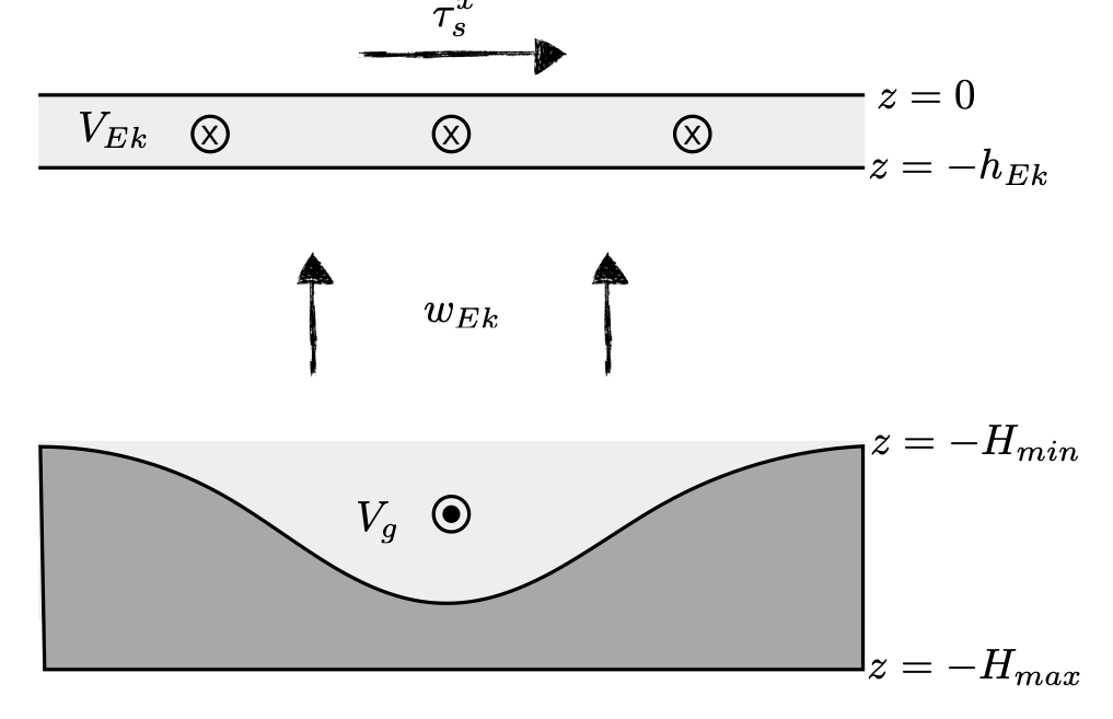
Fig. 2 View of the barotropic ACC model from the south, looking towards the equator.
The Wind-Driven Overturning
Although we eliminated the coriolis force on the meridional flow (\(-fv\)) from our budget by integrating over the full depth of the water column, \eqref{eq:mom} also tells us a lot about the meridional overturning circulation. Let’s now decompose the vertical integral into three regions: the surface Ekman layer, the interior below the Ekman layer and above the topography, and the abyss below the topographic level.
where \(\ab{V_{Ek}}\) is the zonally averaged Ekman transport and \(\ab{V_g}\) is the zonally averaged geostrophic transport below topography. Mass conservation can be expressed as \(\ab{V_{Ek}} + \ab{V_g} = 0\); the Ekman transport near the surface must be returned by an equal and opposite geostrophic flow in the abyss.
The zonal wind stress is not constant with latitude, but rather decreases southward over the ACC latitudes from its maximum around 50S. This means that \(\ab{V_{Ek}}\) also decreases southward, and Ekman pumping is required to supply mass from below. This implies a zonal-mean overturning circulation as shown in Fig.~\ref{fig:cartoon_side}. Mass conservation of the zonally-averaged flow means that \(\partial \ab{v} / \partial y + \partial \ab{w} / \partial z\). Consequently, we can express the overturning circulation using a single scalar {\em streamfunction}:
In the ocean interior (i.e.~\(-H_{max} < z < h_{Ek}\)),
The subscript \(_{Ek}\) reminds us that this overturning circulation is fundamentally wind driven and proportional to the Ekman transport.
Stratification and Eddy Flux
This wind-driven overturning circulation \(\psi_{Ek}\) describes very strong upwelling in the ACC latitudes. Using typical values of wind stress and other parameters, we can estimate \(w_{Ek} \simeq 2.5 \times 10^{-6}\) m/s or about 75 m / year. This upwelling takes place over a strong stratified pycnocline. The question therefore arises: how is this strong advective flux of buoyancy balanced?
In our discussion of advection and diffusion, we considered a one-dimensional balance between vertical advection and diffusion. The zonally-averaged version of this balance is
We found that such a system can be satisfied by a profile of the form
where \(z^\ast = \kappa_v / \ab{w}\) is a scale depth parameter, describing how rapidly the stratification changes with depth.
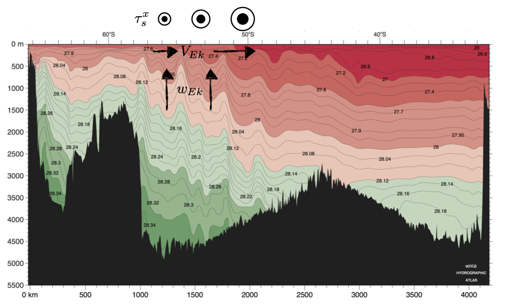
Fig. 3 Neutral density surfaces in the Southern Indian Ocean (WOCE line I8), superimposed with arrows showing the sense of the wind-driven Ekman circulation.
One important characteristic of the Southern Ocean is the relatively deep scale depth of both its stratification and associated thermal wind currents. A section of density in the Southern Indian Ocean (Fig. \ref{fig:gamma}) illustrates this well. An exponential profile is actually not a bad fit; the “scale depth” can be estimated to be approx.~800 m. Plugging in our estimate of \(w_{Ek} \simeq 2.5 \times 10^{-6}\) m/s implies that a value of \(\kappa_v \simeq 2 \times 10^{-3}\) m s\(^{-2}\) would be required to satisfy the balance in \eqref{eq:b1d}. Clearly such a value is far beyond the typical level of turbulent mixing in the thermocline (\(\kappa_v \simeq 1 \times 10^{-5}\) m s\(^{-2}\)). Therefore another mechanism is required to balance the wind-driven vertical advection of buoyancy.
That other mechanism is widely believed to be mesoscale eddy transport. It turns out that \eqref{eq:b1d} is an inadequate description of the buoyancy budget in the Southern Ocean; it neglects strong correlations between transient and small-scale motions which can contribute substantial buoyancy fluxes. To understand how these correlations arise, we must use a buoyancy budget that properly accounts for eddy fluxes.
We start by taking a time and zonal average of \eqref{eq:b}. After some algebra, we can reduce the result to
where
are the eddy fluxes of buoyancy in the meridional and zonal directions. We have introduced the symbol \(\ol{( \ )}\) to indicate a time average. The deviations from the time average are indicated by a prime, and the deviations from the time and zonal average are indicated by a dagger, i.e.
The prime terms are associated with {\em transient} eddy fluctuations (turbulent flow), while the dagger terms are associated with {\em stationary} eddies, a.k.a.~steady meanders of the ACC. Both types of motion can transport buoyancy meridionally and vertically. If the zonal average is reinterpreted as a “streamwise” average around a circumpolar contour which follows the ACC path, the dagger terms will vanish. In practice, the buoyancy budget is generally dominated by the vertical flux terms, i.e.
In our discussion of advection and diffusion, we learned that mesoscale eddies tend to transport properties {\em along} rather than across isopycnals. This results from fundamental dynamical and energetic constrains on the eddy motion. As a result, the eddy buoyancy flux is oriented {\em perpendicular} to the mean buoyancy gradient, i.e.
When \eqref{eq:adiabatic} is satisfied, the eddy fluxes are usually termed “adiabatic.” Given this fact, an ingenious way to simplify \eqref{eq:b1} emerges if we make the following definitions:
and
Using \eqref{eq:adiabatic}, we can now write \eqref{eq:b1} as
In \eqref{eq:psi_eddy}, we defined an {\em eddy-induced} overturning streamfunction \(\psi_{eddy}\). We then defined a {\em residual} overturning streamfunction \(\psi_{res}\) as the sum of this and the wind-driven overturning. What this means is that, when the eddy fluxes are adiabatic and \eqref{eq:adiabatic} is satisfied, we can represent their contribution to the buoyancy budget as {\em advection}, not diffusion! The eddy-induced overturning has the opposite sense as the wind-driven component; hence the net overturning is a small residual (\(\psi_{res}\) between the two opposing terms.
It was clear that the wind stress determines \(\psi_{Ek}\), but it is not so clear what determines \(\psi_{res}\). In general this is a difficult problem, since in involves mesoscale eddy turbulence. However, there is one powerful constraint we can use: the air-sea buoyancy flux.
Assume there is a surface mixed layer of depth \(h_m > h_{Ek}\), within which \(\partial b / \partial z = 0\). At the surface (\(z=0\)), both \(\psi_{Ek}\) and \(\psi_{eddy}\) go to zero. We will further assume that \(B\), the vertical buoyancy flux due to mixing, is vanishingly small in the interior—this is consistent with weak values of \(\kappa_v\) that have been measured in the upper Southern Ocean. We can then integrate \eqref{eq:bres} in the vertical over the surface mixed layer to find
where \(b_s\) is the surface buoyancy and \(B_s\) is the surface air-sea buoyancy flux.
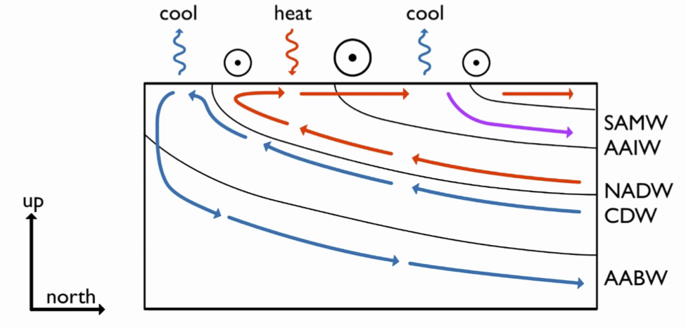
Fig. 4 Idealized view of Southern Ocean residual circulation and mixing