Wind Driven Circulation
Ekman Layers
The low-Rossby-number equations for the ageostrophic flow are given by the balance between the Coriolis term and the friction term:
Frictional effects are mostly important near the top and bottom of the ocean, where the flow rubs agains the boundaries or is exposed to the wind. Technically, the right-hand side of this equation represents molecular viscosity, representing the frictional transfer of momentum by molecules jostling against each other. However, when looking at large scale phenomena, we replace the molecular viscosity with turbulent viscosity, representing the transfer of momentum by turbulent eddies. For Ekman layers, we mostly care about the vertical transfer of momentum. The equations then become.
where \(A_z\) is the turbulent viscosity coefficient (analagous to \(K_z\) in the tracer equations).
Let’s now consider the layer at the top of the ocean. Winds push on the ocean, exerting stress and inducing waves and turbulence. These waves and turbulence help transmit the stress downwards through the water column, effectively “mixing” the momentum from the winds over a broader layer than just the surface itself. But eventually, if you go deep enough, the wind-driven turbulence dies out. At this point, you have reached the bottom of the Ekman layer, the boundary layer over which frictional momentum is mixed.
How deep is the Ekman layer? It is possible to solve the equations exactly, but we will not go through the full solution in this course. The Ekman layer depth turns out to be given by
We can understand this depth scale in the following way: is represents the distance momentum can travel vertically due to turbulent mixing before it feels the influence of the coriolis force.
Below the Ekman layer, the frictional transfer of momentum vanishes (by construction). We can use this fact to develop an integral view of the Ekman layer by integrating in the vertical. First, we express the frictional momentum balance using a cross product:
Now we integrate in the vertical to obtain
The second term on the RHS is zero because it represents the frictional transfer of momentum at the base of the Ekman layer. The first term is the frictional stress at the top of the ocean: this is equal to the stress imparted by the wind
(appropriately scaled by the Boussinesq reference density).
The quantity on the LHS is defined as the Ekman Transport:
It has units of m\(^2\) s\(^{-1}\) and represents the net horizontal transport with the Ekman layer. We can rearragnge the equation to read:
This equation shows that the Ekman transport is always to the right of the wind stress (in the Northern Hemisphere). In component form, it reads:
Ekman Pumping
Mass conservation states that water must be upwelled or downwelled to / from the Ekman layer in order to supply the Ekman transport. The Boussinesq volume conservation equation states that:
Integrating over the Ekman layer, and neglecting the small volume flux in/out of the ocean surface due to evaporation and precipitation, gives
The vertical velocity at the base of the Ekman layer is called the Ekman pumping. Substituting the Ekman transport in this equation, we obtain
This can also be written as a curl:
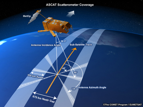
Measuring Winds with Scatterometry
 http://www.eumetrain.org/data/2/227/navmenu.php?tab=&page=1.2.0
SCOW: http://cioss.coas.oregonstate.edu/scow/
import xarray as xr
import numpy as np
from matplotlib import pyplot as plt
%matplotlib inline
scow = xr.open_dataset('http://wilson.coas.oregonstate.edu:8080/thredds/dodsC/CIOSS/SCOW/Monthly/scow_monthly_maps.nc')
scow
<xarray.Dataset>
Dimensions:                      (latitude: 560, longitude: 1440, time: 12)
Coordinates:
  * latitude                     (latitude) float32 -69.875 -69.625 -69.375 ...
  * longitude                    (longitude) float32 0.125 0.375 0.625 0.875 ...
  * time                         (time) datetime64[ns] 2001-01-01 ...
Data variables:
    scow_wind_curl               (time, longitude, latitude) float64 ...
    scow_wind_divergence         (time, longitude, latitude) float64 ...
    scow_wind_stress_curl        (time, longitude, latitude) float64 ...
    scow_wind_stress_divergence  (time, longitude, latitude) float64 ...
    scow_zonal_wind_stress       (time, longitude, latitude) float64 ...
    scow_meridional_wind_stress  (time, longitude, latitude) float64 ...
    scow_wind_stress_magnitude   (time, longitude, latitude) float64 ...
    scow_zonal_wind              (time, longitude, latitude) float64 ...
    scow_meridional_wind         (time, longitude, latitude) float64 ...
    scow_wind_speed              (time, longitude, latitude) float64 ...
    scow_wind_speed_squared      (time, longitude, latitude) float64 ...
    scow_wind_speed_cubed        (time, longitude, latitude) float64 ...
    amsr_sst                     (time, longitude, latitude) float64 ...
    avhrr_sst                    (time, longitude, latitude) float64 ...
Attributes:
    title:                      Scatterometer Climatology of Ocean Winds (SCO...
    summary:                    This data set contains monthly, global SCOW f...
    author:                     Craig Risien (crisien@coas.oregonstate.edu)
    institution:                Oregon State University, College of Earth, Oc...
    date_created:               2017-02-15T16:54:28
    history:                    From the updated Risien and Chelton 2008 SCOW...
    keywords:                   SCOW monthly wind QuikSCAT global AMSR AVHRR ...
    keyword_vocabulary:         GCMD
    reference:                  Risien, C.M., and D.B. Chelton, 2008: A Globa...
    Conventions:                CF-1.6
    comments:                   The original SCOW climatology (Risien and Che...
    geospatial_lat_min:         -90.0
    geospatial_lat_max:         90.0
    geospatial_lat_units:       degrees_north
    geospatial_lat_resolution:  0.25 degree grid
    geospatial_lon_min:         0.0
    geospatial_lon_max:         360.0
    geospatial_lon_units:       degrees_east
    geospatial_lon_resolution:  0.25 degree grid
    source:                     QuikSCAT observations
    standard_name_vocabulary:   CF Standard Name Table v32
    references:                 http://journals.ametsoc.org/doi/abs/10.1175/2...
    cdm_data_type:              grid
    sensor:                     QuikSCAT
    license:                    These data are available for use without rest...
# create an annual mean -- takes a long time to load data
scow_am = scow.mean(dim='time').load()
ds = scow_am.transpose('latitude', 'longitude')
omega = 7.29e-5
f = 2 * omega * np.sin(np.deg2rad(ds.latitude))
rho0 = 1030
ds['U_ek'] = ds.scow_meridional_wind_stress / (rho0 * f).where(abs(ds.latitude)>5)
ds['V_ek'] = -ds.scow_zonal_wind_stress / (rho0 * f).where(abs(ds.latitude)>5)
def quick_quiver(u, v, sampling_x=10, sampling_y=10, mag_max=None, **kwargs):
    x = u.longitude
    y = u.latitude
    mag = 0.5*(u**2 + v**2)**0.5
    slx = slice(None, None, sampling_x)
    sly = slice(None, None, sampling_y)
    sl2d = (sly, slx)
    fig, ax = plt.subplots(**kwargs)
    mag.plot(ax=ax, vmax=mag_max)
    return ax, ax.quiver(x[slx], y[sly], u[sl2d], v[sl2d])
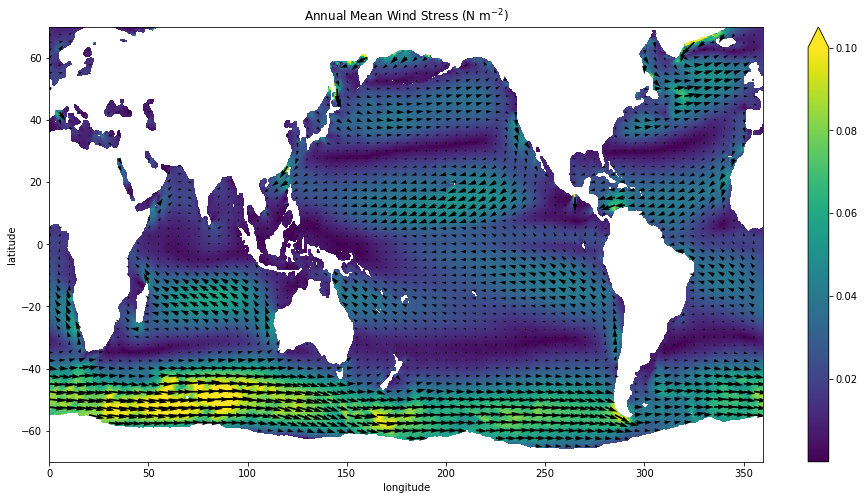
quick_quiver(ds.scow_zonal_wind_stress, ds.scow_meridional_wind_stress,
             mag_max=0.1, sampling_x=20, figsize=(16,8))
plt.title(r'Annual Mean Wind Stress (N m$^{-2}$)');
<matplotlib.text.Text at 0x1bdce4390>
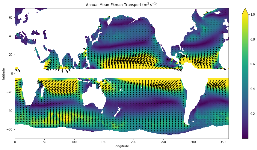
quick_quiver(U_ek, V_ek, mag_max=1,
             sampling_x=20, figsize=(16,8))
plt.title(r'Annual Mean Ekman Transport (m$^{2}$ s$^{-1}$)');
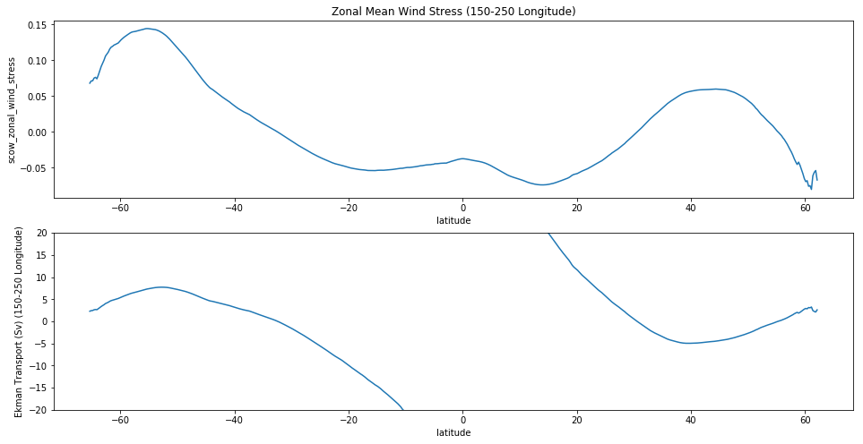
fig, (ax1, ax2) = plt.subplots(nrows=2, figsize=(16,8))
(ds.scow_zonal_wind_stress
    .sel(longitude=slice(150,250))
    .mean(dim='longitude')
    .plot(ax=ax1))
((V_ek * (110e3 * 100 * np.cos(np.deg2rad(ds.latitude)))/1e6)
    .sel(longitude=slice(150,250))
    .mean(dim='longitude')
    .plot(ax=ax2))
ax1.set_title('Zonal Mean Wind Stress (150-250 Longitude)')
ax2.set_ylim(-20, 20)
ax2.set_ylabel('Ekman Transport (Sv) (150-250 Longitude)')
<matplotlib.text.Text at 0x1e74c7d68>
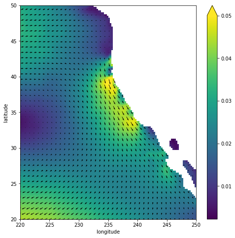
Coastal Upwelling
cal = ds.sel(longitude=slice(220, 250), latitude=slice(20,50))
quick_quiver(cal.scow_zonal_wind_stress, cal.scow_meridional_wind_stress,
             mag_max=0.05, sampling_x=3, sampling_y=3, figsize=(8,8));
(<matplotlib.axes._subplots.AxesSubplot at 0x1e43143c8>,
 <matplotlib.quiver.Quiver at 0x18674d048>)
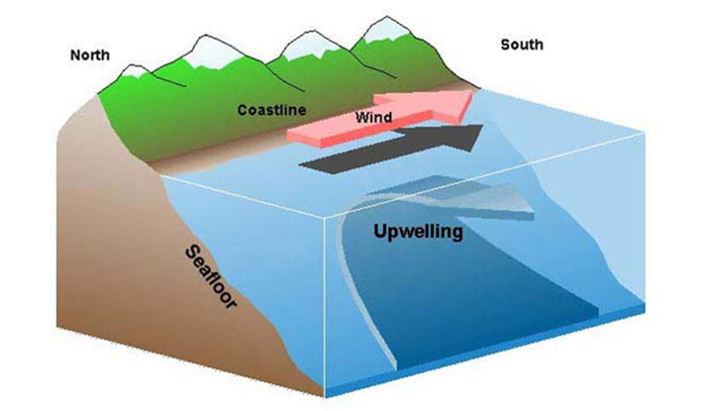
Via https://oceanexplorer.noaa.gov/facts/upwelling.html
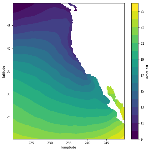
plt.figure(figsize=(8,8))
cal.avhrr_sst.plot.contourf(levels=20)
<matplotlib.contour.QuadContourSet at 0x1e69294a8>
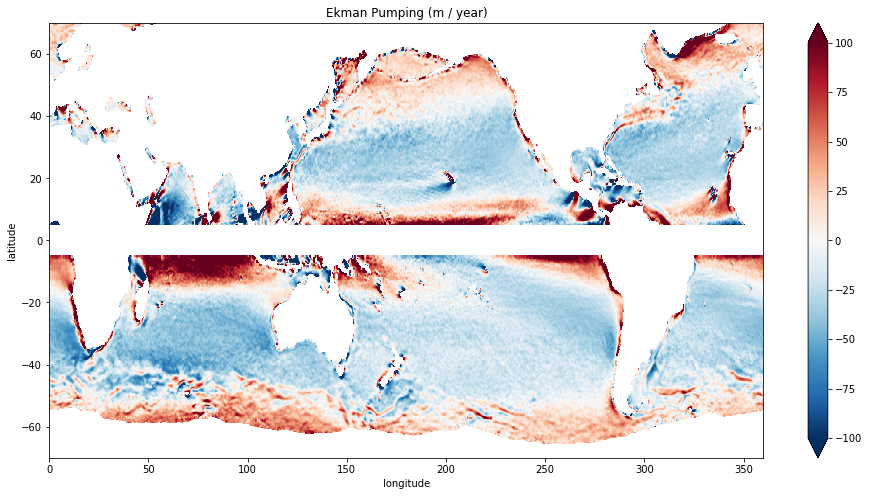
Global Ekman Pumping
# this is only approximate...f should be inside the curl
w_ek = (ds.scow_wind_stress_curl / (rho0 * f) / 1e7).where(abs(ds.latitude)>5)

plt.figure(figsize=(16,8))
(w_ek * 24*60*60*364).plot(vmax=100)
plt.title('Ekman Pumping (m / year)')
<matplotlib.text.Text at 0x1e6831588>