Vorticity, Sverdrup Transport, and Ocean Gyres¶

Vorticity¶

We begin with the general definition of vorticity, which is an important concept for ocean circulation theory. Despite its importance, it can be hard to develop and intuitive understanding of vorticity. Here is my best attempt at a definition in normal language

Vorticity represents the local “spinniness” of a point in the fluid.

Vorticity is, in general, a vector, defined as the curl of the velocity field.

\[ \boldsymbol{\omega} = \nabla \times \mathbf{u} \]

The unadorned symbol $\boldsymbol{\omega}$ is the relative vorticity, measured by the observer in the rotating reference frame. If measuring vorticity from the intertial reference frame, we would also measure the component due to the Earth’s rotation itself, the “spinniness” of the Earth. This is the absolute vorticity:

\[ \boldsymbol{\omega}_a = \nabla \times \mathbf{u} + \boldsymbol{\Omega} = \boldsymbol{\omega} + \boldsymbol{\Omega} \]

For large scale ocean circulation, we are usually only concerned with the horizontal flow, i.e.~the flow in the plane tangent to the Earth’s surface. We denote this as

\[ \omega = \hat{\mathbf{k}} \cdot \boldsymbol{\omega} = -\pd{u}{y} + \pd{v}{x} \]

Planetary Vorticity Equation¶

In previous lectures, we considered the planetry approximation, in which the horizontal equations of motion reduced to the following form:

\[\begin{split} \begin{align} \pd{u}{t} - f v &= -\pd{\phi}{x} + \frac{1}{\rho_0}\pd{\tau_x}{z} \\ \pd{v}{t} + f u &= -\pd{\phi}{y} + \frac{1}{\rho_0}\pd{\tau_y}{z} \end{align} \end{split}\]

where we have represented the friction terms using a stress $\tau$. Note that we have left the time-dependent term in the equations, despite the small Rossby number. We will drop them again later. For now, they make it easier to answer the question What do the planetary equations say about vorticity? To answer this we combine the equations in a way that allows us to write an expression for $\omega$. First we work on the left-hand side of the equations taking $- \partial_y$ of the first and adding this to $\partial_x$ of the second:

\[\begin{split} \begin{align} -\pd{}{y} \left (\pd{u}{t} - f v \right) + \pd{}{x} \left (\pd{v}{t} + f u \right) &= \\ \pd{}{t} \left (-\pd{u}{y} + \pd{v}{x} \right) + \pd{}{y} (fv) + \pd{}{x} (fu) &= \\ \pd{\omega}{t} + f\left ( \pd{u}{x} + \pd{v}{y} \right ) + \beta v &= \end{align} \end{split}\]

(Recall that $\beta = df/dy$.) The continuity equation says that

\[ \pd{u}{x} + \pd{v}{y} + \pd{w}{z} = 0 \]

which allows us to write the left-hand side as

\[ \pd{\omega}{t} - f \pd{w}{z} + \beta v = \ . \]

On the right hand side, we see that the pressure terms cancel

\[ = \pd{^2\phi}{x \partial y} - \pd{^2\phi}{x \partial y} + \frac{1}{\rho_0} \left ( - \pd{}{y}\pd{\tau_x}{z} + \pd{}{x}\pd{\tau_y}{z} \right ) \ . \]

The full vorticity equation can now be written as

\[ \pd{\omega}{t} - f \pd{w}{z} + \beta v = \frac{1}{\rho_0} \pd{}{z} \left ( -\pd{\tau_x}{y} + \pd{\tau_y}{x} \right ) \ . \]

The first term represents the rate of change of vorticity. (For small Rossby number, this time deriviative will be small.)
The second term represents “vortex stretching”: it quantifies how vertical motion, which forces the fluid parcel to expand or contract horizontally, can translate into the production and removal of vorticity. This is relate to the conservation of angular momentum and is similar to how a figure skater accelerates their spinning by contracting their arms and legs.
The third term $\beta v$ represents the production of vorticity due to advection across the planetary vorticity gradient. Effectively, it describes how the planetary vorticity of the spinning earth can be converted to relative vorticity of the water parcel, via a change in latitude of the water parcel.
The term on the right-hand is the curl of the stress divergence. It represents the mechanical torque imposed on the ocean by frictional forces.

In the interior ocean (away from the top and bottom boundaries), the friction will be small, leaving the approximate balance

\[ \beta v = f \pd{w}{z} \]

Barotropic Vorticty¶

The barotropic ocean circuluation is the horizontal flow integrated over the full depth of the ocean. For simplicity, here we will take the ocean to have a uniform depth of $H$. The depth-integrated flow is given by

\[ U, V = \int_{-H}^0 (u, v) dz \]

If we integrate the continuity equation vertically, we find

\[ \pd{U}{x} + \pd{V}{y} + w|_{z=0} - w|_{z=-H} = 0 \ .\]

Neglecting the small contribution of evaporation and precipitation, there is no vertical flow either through the surface or the bottom of the ocean, leaving

\[ \pd{U}{x} + \pd{V}{y} = 0 \ .\]

Because $(U, V)$ is a two-dimensional non-divergent flow, we can represent is using a streamfunction $\Psi$, defined as

\[ U = -\pd{\Psi}{y} \ , \ \ V = \pd{\Psi}{x} \ . \]

This notation simplifies our description of the barotropic circulation.

The barotropic vorticity $Z$ is defined as

\[ Z = -\pd{U}{y} + \pd{V}{x} = \nabla^2 \Psi \ . \]

To obtain an equation for $Z$, we just take the vertical integral of the planetry vorticity equation. We obtain

\[ \pd{Z}{t} + \beta V = \frac{1}{\rho_0} \left ( -\pd{\tau_x}{y} + \pd{\tau_y}{x} \right )_{z=0} - \frac{1}{\rho_0} \left ( -\pd{\tau_x}{y} + \pd{\tau_y}{x} \right )_{z=-H}\ . \]

Disregarding the tendency term, we can write this compactly as

\[ \beta V = \frac{1}{\rho_0} \left [ \mbox{curl} ( \boldsymbol{\tau}_{surf}) - \mbox{curl} (\boldsymbol{\tau}_{bot}) \right ] \]

where curl $= \hat{\mathbf{k}} \cdot \nabla \times$ represents the curl of the vector in the horizontal plane. This equation shows us that the barotropic meridional flow $V$ is proportional to the curl of the frictional boundary stresses on the ocean. There is a contribution to the stress from the surface (wind stress) and the bottom (drag). However, over most of the ocean, the deep flow is very weak, meaning that bottom drag is negligible. In this case, the barotropic vorticity equation reduces to the form that is commonly called Sverdrup Balance:

\[ \beta V_{Sv} = \frac{1}{\rho_0} \mbox{curl} ( \boldsymbol{\tau}_{surf}) \ . \]

Sverdrup balance is a remarkable simplification of the ocean circulation. It tells us that, just given knowledge of the wind stress field, we can predict the full-depth integrated meridional transport.

Topographic Beta Effect¶

In our laboratory experiment $f$ is constant ($f_0$). However, we have a sloping bottom, such that $d H/d y = s_y$. The bottom boundary condition is no longer $w=0$. Instead, it is $\mathbf{u} \cdot \nabla H + w = 0$. If we assume the horizontal flow is barotropic (uniform with depth), we obtain

\[ w|_{z=-H} = \frac{s_y}{H} V \]

Using this when we vertically integrate the vorticity equations gives

\[ \pd{Z}{t} + \frac{f_0 s_y}{H} V = \frac{1}{\rho_0} \left ( -\pd{\tau_x}{y} + \pd{\tau_y}{x} \right )_{z=0} - \frac{1}{\rho_0} \left ( -\pd{\tau_x}{y} + \pd{\tau_y}{x} \right )_{z=-H}\ . \]

The factor

\[ f_0 s_y / H \equiv \beta_{eff} \]

plays the same mathematical role as $\beta$ on the rotating sphere. The topographic Sverdrup balance is

\[ \beta_{eff} V_{Sv} = \frac{1}{\rho_0} \mbox{curl} ( \boldsymbol{\tau}_{surf}) \ . \]

import xarray as xr
import numpy as np
from matplotlib import pyplot as plt
%matplotlib inline

scow = xr.open_dataset('http://wilson.coas.oregonstate.edu:8080/thredds/dodsC/CIOSS/SCOW/Monthly/scow_monthly_maps.nc')
scow

<xarray.Dataset>
Dimensions:                      (latitude: 560, longitude: 1440, time: 12)
Coordinates:
  * latitude                     (latitude) float32 -69.875 -69.625 -69.375 ...
  * longitude                    (longitude) float32 0.125 0.375 0.625 0.875 ...
  * time                         (time) datetime64[ns] 2001-01-01 ...
Data variables:
    scow_wind_curl               (time, longitude, latitude) float64 ...
    scow_wind_divergence         (time, longitude, latitude) float64 ...
    scow_wind_stress_curl        (time, longitude, latitude) float64 ...
    scow_wind_stress_divergence  (time, longitude, latitude) float64 ...
    scow_zonal_wind_stress       (time, longitude, latitude) float64 ...
    scow_meridional_wind_stress  (time, longitude, latitude) float64 ...
    scow_wind_stress_magnitude   (time, longitude, latitude) float64 ...
    scow_zonal_wind              (time, longitude, latitude) float64 ...
    scow_meridional_wind         (time, longitude, latitude) float64 ...
    scow_wind_speed              (time, longitude, latitude) float64 ...
    scow_wind_speed_squared      (time, longitude, latitude) float64 ...
    scow_wind_speed_cubed        (time, longitude, latitude) float64 ...
    amsr_sst                     (time, longitude, latitude) float64 ...
    avhrr_sst                    (time, longitude, latitude) float64 ...
Attributes:
    title:                      Scatterometer Climatology of Ocean Winds (SCO...
    summary:                    This data set contains monthly, global SCOW f...
    author:                     Craig Risien (crisien@coas.oregonstate.edu)
    institution:                Oregon State University, College of Earth, Oc...
    date_created:               2017-02-15T16:54:28
    history:                    From the updated Risien and Chelton 2008 SCOW...
    keywords:                   SCOW monthly wind QuikSCAT global AMSR AVHRR ...
    keyword_vocabulary:         GCMD
    reference:                  Risien, C.M., and D.B. Chelton, 2008: A Globa...
    Conventions:                CF-1.6
    comments:                   The original SCOW climatology (Risien and Che...
    geospatial_lat_min:         -90.0
    geospatial_lat_max:         90.0
    geospatial_lat_units:       degrees_north
    geospatial_lat_resolution:  0.25 degree grid
    geospatial_lon_min:         0.0
    geospatial_lon_max:         360.0
    geospatial_lon_units:       degrees_east
    geospatial_lon_resolution:  0.25 degree grid
    source:                     QuikSCAT observations
    standard_name_vocabulary:   CF Standard Name Table v32
    references:                 http://journals.ametsoc.org/doi/abs/10.1175/2...
    cdm_data_type:              grid
    sensor:                     QuikSCAT
    license:                    These data are available for use without rest...

# create an annual mean -- takes a long time to load data
scow_am = scow.mean(dim='time').load()
ds = scow_am.transpose('latitude', 'longitude')

def quick_quiver(u, v, sampling_x=10, sampling_y=10,
                 scalar=None, mag_max=None, **kwargs):
    x = u.longitude
    y = u.latitude
    slx = slice(None, None, sampling_x)
    sly = slice(None, None, sampling_y)
    sl2d = (sly, slx)
    if scalar is None:
        mag = 0.5*(u**2 + v**2)**0.5
    else:
        mag = scalar

    fig, ax = plt.subplots(**kwargs)
    mag.plot(ax=ax, vmax=mag_max)
    return ax, ax.quiver(x[slx], y[sly], u[sl2d], v[sl2d])

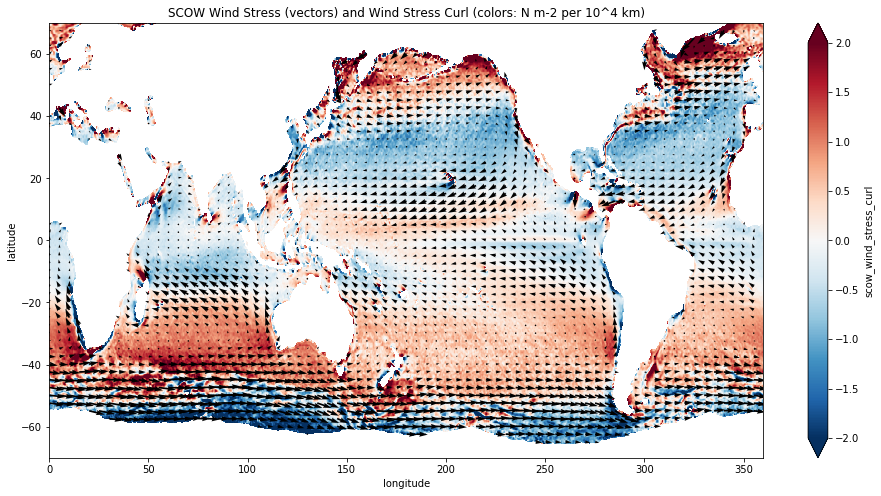
quick_quiver(ds.scow_zonal_wind_stress, ds.scow_meridional_wind_stress,
             scalar=ds.scow_wind_stress_curl,
             mag_max=2, sampling_x=20,
             figsize=(16,8))
plt.title(r'SCOW Wind Stress (vectors) and Wind Stress Curl (colors: %s)' 
           % scow.scow_wind_stress_curl.attrs['units']);

_images/vorticity_sverdrup_transport_and_gyres_9_0.png

omega = 7.29e-5
R = 6.3781e6
f = 2 * omega * np.sin(np.deg2rad(ds.latitude))
beta = 2 * omega / R * np.cos(np.deg2rad(ds.latitude))
rho0 = 1030
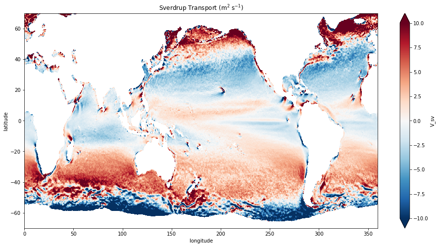
ds['V_sv'] = ds.scow_wind_stress_curl / (beta * rho0 * 1e7)

fig, ax = plt.subplots(figsize=(16,8))
ds.V_sv.plot(vmax=10, ax=ax)
plt.title(r'Sverdrup Transport (m$^2$ s$^{-1}$)')

<matplotlib.text.Text at 0x1159eae48>

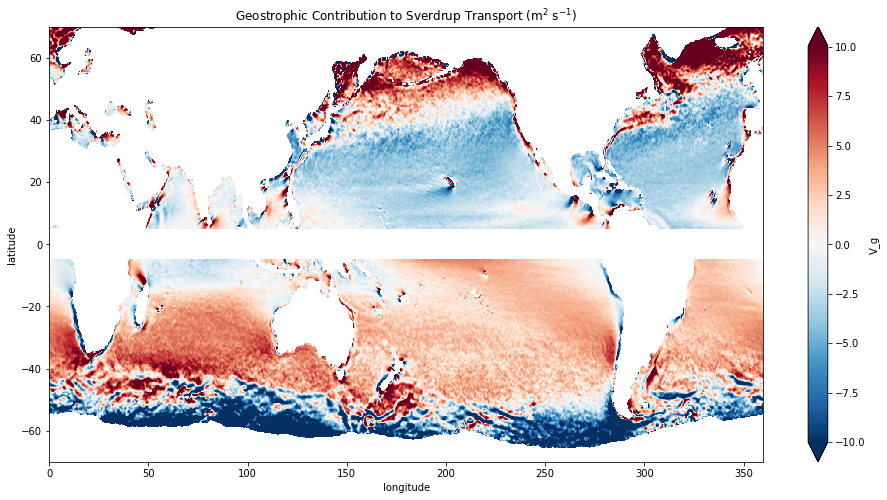
_images/vorticity_sverdrup_transport_and_gyres_11_1.png

Ekman and Geostrophic Contributions to Sverdrup Transport¶

Under the planetary approximation, the Sverdrup transport is composed of both Ekman and geosptrophic contributions:

\[ V_{Sv} = V_{Ek} + V_g \ . \]

In the previous lecture, we saw that

\[ V_{Ek} = -\frac{\tau_x}{\rho_0 f} \ . \]

This, together with the Sverdrup transport, determines the amount of flow carried by the geostrophic flow:

\[ V_g = \frac{1}{\rho_0 \beta} \mbox{curl} ( \boldsymbol{\tau}_{surf}) + \frac{\tau_x}{\rho_0 f} \]

ds['V_ek'] = -ds.scow_zonal_wind_stress / (rho0 * f).where(abs(ds.latitude)>5)
ds['V_g'] = ds.V_sv - ds.V_ek

fig, ax = plt.subplots(figsize=(16,8))
ds.V_g.plot(vmax=10, ax=ax)
plt.title(r'Geostrophic Contribution to Sverdrup Transport (m$^2$ s$^{-1}$)')

<matplotlib.text.Text at 0x18ae332b0>

_images/vorticity_sverdrup_transport_and_gyres_14_1.png

Calculation of the Streamfunction¶

Once we know $V$ (using Sverdrup balance), we can use mass continuity to determine $U$, via the sverdrup balance.

The constraint that there be no normal flow across the ocean’s horizontal boundaries means that $\Psi = const$ on the boundaries. We pick this constant aribtrarily to be 0. We know $V = \partial \Psi / \partial x$. We integrate this in $x$ to obtain

\[ \int_{x_1}^{x_2} V_{Sv} dx = \Psi(x_2, y) - \Psi(x_1, y) \]

If we choose either $x_1$ or $x_2$ on the ocean boundary (where $\Psi=0$), we have determined $\Psi$ at an arbitrary point in the interior. However, we must choose whether to choose the eastern or western boundary as the limit of integration. This cannot be determined by Sverdrup balance alone; it requires conisderation of frictional boundary layers.

We will see below that conservation of vorticity requires us to choose the eastern boundary, requiring closure of the circulation in a western boundary current. We accept this for now and set $x_2 = x_e$ (the longitude of the eastern boundary). We require that the streamfunction be zero on the eastern boundary, i.e. $\Psi(x_e, y) = 0$. To find the value of the streamfunction in the interior at any point in $x$, we let $x_1$, the western limit of the integral, become $x$, and perform the integration over dummy variable $x'$:

\[ \Psi(x, y) = - \int_{x}^{x_e} V_{Sv}(x', y) dx' . \]

Equivalently, we can integrate from the eastern boundary to find

\[ \Psi(x, y) = \int_{x_e}^x V_{Sv}(x', y) dx' \ . \]

ds.coords['dx'] = (R * np.cos(np.deg2rad(ds.latitude))
                   * np.deg2rad(ds.longitude.diff(dim='longitude')))

def plot_sverdrup_streamfunction(ds, levels=20, **kwargs):
    psi = -(ds.V_sv * ds.dx).isel(longitude=slice(None,None,-1)).cumsum(dim='longitude')/1e6
    psi = psi.where(~ds.V_sv.isnull())
    
    fig, ax = plt.subplots(**kwargs)
    psi.plot.contourf(levels=levels)
    return psi

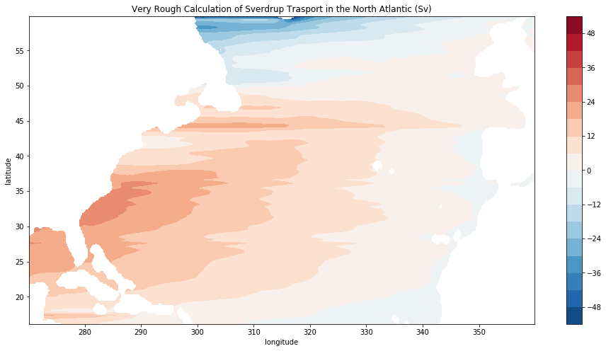
ds_natl = ds.sel(longitude=slice(270, 360), latitude=slice(16, 60)) 
plot_sverdrup_streamfunction(ds_natl, figsize=(16,8))
plt.title('Very Rough Calculation of Sverdrup Trasport in the North Atlantic (Sv)')

<matplotlib.text.Text at 0x180b26ba8>

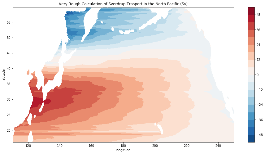
_images/vorticity_sverdrup_transport_and_gyres_16_1.png

ds_npac = ds.sel(longitude=slice(110, 250), latitude=slice(16, 60))
psi_npac = plot_sverdrup_streamfunction(ds_npac, figsize=(16, 8))
plt.title('Very Rough Calculation of Sverdrup Trasport in the North Pacific (Sv)')

<matplotlib.text.Text at 0x18a108898>

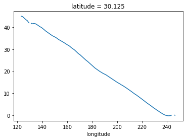
_images/vorticity_sverdrup_transport_and_gyres_17_1.png

psi_npac.sel(latitude=30, method='nearest').plot()

[<matplotlib.lines.Line2D at 0x18b4b63c8>]

_images/vorticity_sverdrup_transport_and_gyres_18_1.png

Boundary Currents¶

We have neglected bottom friction so far. This is fine in the open ocean. However, in order to close the circulation, we need to invoke friction within a narrow boundary layer. We will use the simplest possible form of friction: linear bottom drag. With linear bottom drag, the frictional stress at the bottom is given by

\[ \frac{1}{\rho_0} \boldsymbol{\tau}_{bot} = R \mathbf{U} \]

where $r$ represents the rate at which bottom friction retards the barotropic flow.

The full barotropic vorticity equation then becomes

\[ \beta V = \frac{1}{\rho_0} \mbox{curl} ( \boldsymbol{\tau}_{surf}) - R \left ( -\pd{U}{y} + \pd{V}{x} \right ) \]

or

\[ R \nabla^2 \Psi + \beta \pd{\Psi}{x} = \frac{1}{\rho_0} \mbox{curl} ( \boldsymbol{\tau}_{surf} ) \ . \]

(This is sometimes called Stommel’s equation.) We can split it up into a Sverdrup component (defined above), and a boundary current component, defined as:

\[ R \nabla^2 \Psi_{bc} + \beta \pd{\Psi_{bc}}{x} = 0 \ . \]

Note that we have used only the boundary current in the laplacian under the assumption that the Sverdrup flow does not have enough curvature to make a significant contribution to the first term in the equation.

If we integrate this equation in longitude across the entire basin, we obtain $$ R \int_{x_w}^{x_e} \nabla^2 \Psi dx = \int_{x_w}^{x_e} \frac{1}{\rho_0} \mbox{curl} ( \boldsymbol{\tau}_{surf} ) dx \ . $$

Assuming that the boundary current flows mostly in the meridional direction, we can simplify this to

\[ R \delta \ol{\pd{V}{x}} \simeq \int_{x_w}^{x_e} \frac{1}{\rho_0} \mbox{curl} ( \boldsymbol{\tau}_{surf} ) dx \ . \]

Intro to Physical Oceanography