Air Sea Exchange
import xarray as xr
from matplotlib import pyplot as plt
import numpy as np
import gsw
import pooch
import cartopy.crs as ccrs
import hvplot.xarray
import hvplot.pandas
import re
%matplotlib inline
%config InlineBackend.figure_format = 'retina'
plt.rcParams['figure.figsize'] = (15,9)
plt.rcParams['font.size'] = 16
#plt.rcParams['lines.linewidth'] = 3
from IPython.display import SVG, display, Image, display_svg, YouTubeVideo
opts = dict(geo=True, frame_width=800, frame_height=420, projection=ccrs.Robinson(), coastline=True, legend=False ,features={'land': '110m'})
As anyone who has been to sea knows, the interface between ocean and atmosphere can be an incredibly violent place. Within a hurricane, for example, it is in fact impossible to draw a clear boundary between ocean and atmosphere; the extreme winds whip up a continuous emulsion of air and water. Nevertheless, outside of such extreme cases, there exist robust and relatively simple equations for describing the exchange of heat, freshwater, and momentum between atmosphere and ocean.
display(YouTubeVideo("BhduxaGtNJ8", width=640, height=480))
Atmospheric Circulation
Although this is an oceanography class, this topic requires us to know a bit about the atmosphere. We must have some grasp of the patterns of global atmospheric circulation in order to interpret the patterns of cloud, precipitation, and evaporation which influence air-sea interaction.
Hadley Circulation
The large-scale atmospheric circulation is shown in this figure:

Kaidor, CC BY-SA 3.0 https://creativecommons.org/licenses/by-sa/3.0, via Wikimedia Commons
Major important feature of the global circulation include:
Two overturning ciruclation cells (Hadley Cells) centered around the equator:
Strong ascent near the equator (Intertropical Convergence Zone; ITCZ), which drives precipitation and cloud cover.
Strong descent in the extratropics. The descending air comes from high in the atmosphere and is thus very dry. As a result, there is little rain and atmospheric moisture at these latitudes. This is why we have deserts.
Strong westerly winds in midlatitudes
Strong synoptic-scale storms in midlatitudes. These storms bring heavy wind gusts and precipitation to higher latitudes.
The Mixed Layer
Our starting point is to consider the ocean surface mixed layer and its coupling with the atmosphere. An important property of the surface ocean is that it nearly always contains a layer of well-mixed (i.e. vertically homogeneous) water overlying the stratified interior (the thermocline / pycnocline). This is illustrated in the ARGO profiles shown below.
import fsspec
url = 'https://www.ncei.noaa.gov/data/oceans/argo/gadr/data/atlantic/2015/09/nodc_D1901358_079.nc'
with fsspec.open(url) as fp:
argo = xr.open_dataset(fp).isel(n_prof=0).load()
argo['s_a'] = gsw.SA_from_SP(argo.psal, argo.pres, argo.longitude, argo.latitude)
argo['c_t'] = gsw.CT_from_t(argo.s_a, argo.temp, argo.pres)
argo['rho'] = gsw.rho(argo.s_a, argo.c_t, argo.pres)
argo['sig0'] = gsw.sigma0(argo.s_a, argo.c_t)
argo['sig2'] = gsw.sigma2(argo.s_a, argo.c_t)
argo['sig4'] = gsw.sigma4(argo.s_a, argo.c_t)
Nsquared, p_mid = gsw.Nsquared(argo.s_a, argo.c_t, argo.pres)
argo_p = argo.swap_dims({'n_levels': 'pres'})
argo_p
<xarray.Dataset>
Dimensions: (n_calib: 1, n_history: 4, n_param: 3, pres: 77)
Coordinates:
* pres (pres) float32 6.2 10.3 ... 1.9e+03 1.95e+03
Dimensions without coordinates: n_calib, n_history, n_param
Data variables: (12/70)
data_type object b'Argo profile '
format_version object b'3.1 '
handbook_version object b'1.2 '
reference_date_time object b'19500101000000'
date_creation object b'20161104225754'
date_update object b'20170714162347'
... ...
s_a (pres) float64 36.52 36.52 36.52 ... 35.1 35.1
c_t (pres) float64 22.69 22.68 ... 3.299 3.239
rho (pres) float64 1.025e+03 ... 1.037e+03
sig0 (pres) float64 25.03 25.04 ... 27.8 27.81
sig2 (pres) float64 33.39 33.39 ... 36.93 36.94
sig4 (pres) float64 41.39 41.39 ... 45.66 45.67
Attributes: (12/49)
title: Argo float vertical profile
institution: CORIOLIS
source: Argo float
history: 2018-06-09T01:59:23Z csun convAGDAC.f90 ...
references: http://www.nodc.noaa.gov/argo/
user_manual_version: 3.1
... ...
time_coverage_end: 2015-09-07T12:29:26Z
time_coverage_duration: point
time_coverage_resolution: point
gadr_ConventionVersion: GADR-3.0
gadr_program: convAGDAC.f90
gadr_programVersion: 1.0- n_calib: 1
- n_history: 4
- n_param: 3
- pres: 77
- pres(pres)float326.2 10.3 15.4 ... 1.9e+03 1.95e+03
- long_name :
- Sea water pressure, equals 0 at sea-level
- standard_name :
- sea_water_pressure
- units :
- decibar
- valid_min :
- 0.0
- valid_max :
- 12000.0
- C_format :
- %7.1f
- FORTRAN_format :
- F7.1
- resolution :
- 0.1
- axis :
- Z
array([ 6.2, 10.3, 15.4, 19.9, 25. , 30.2, 35.5, 40.4, 45.1, 49.7, 60.6, 70.9, 80.2, 90.1, 99.4, 109.4, 119.6, 129.7, 139.6, 149.8, 160. , 170.2, 179.3, 189.7, 199.8, 210.4, 220.6, 230.3, 239.9, 250.2, 260.2, 270.3, 280.5, 289.9, 300. , 310. , 320.3, 330.5, 340.1, 350. , 375.5, 399.6, 424.9, 450.1, 474.8, 549.5, 574.8, 599.9, 625.4, 649.6, 675.6, 700.3, 749.6, 800. , 849. , 900.4, 949.5, 999.4, 1050.1, 1100.3, 1150.6, 1200.5, 1249.8, 1300.3, 1349.9, 1400.2, 1450. , 1500. , 1550.1, 1600.3, 1650. , 1700. , 1750.1, 1800.4, 1850.3, 1899.7, 1950. ], dtype=float32)
- data_type()objectb'Argo profile '
- long_name :
- Data type
- conventions :
- Argo reference table 1
array(b'Argo profile ', dtype=object)
- format_version()objectb'3.1 '
- long_name :
- File format version
array(b'3.1 ', dtype=object)
- handbook_version()objectb'1.2 '
- long_name :
- Data handbook version
array(b'1.2 ', dtype=object)
- reference_date_time()objectb'19500101000000'
- long_name :
- Date of reference for Julian days
- conventions :
- YYYYMMDDHHMISS
array(b'19500101000000', dtype=object)
- date_creation()objectb'20161104225754'
- long_name :
- Date of file creation
- conventions :
- YYYYMMDDHHMISS
array(b'20161104225754', dtype=object)
- date_update()objectb'20170714162347'
- long_name :
- Date of update of this file
- conventions :
- YYYYMMDDHHMISS
array(b'20170714162347', dtype=object)
- platform_number()objectb'1901358 '
- long_name :
- Float unique identifier
- conventions :
- WMO float identifier : A9IIIII
array(b'1901358 ', dtype=object)
- project_name()objectb'BSH ...
- long_name :
- Name of the project
array(b'BSH ', dtype=object) - pi_name()objectb'Birgit KLEIN ...
- long_name :
- Name of the principal investigator
array(b'Birgit KLEIN ', dtype=object) - station_parameters(n_param)objectb'PRES ' ... b'PSAL ...
- long_name :
- List of available parameters for the station
- conventions :
- Argo reference table 3
array([b'PRES ', b'TEMP ', b'PSAL '], dtype=object) - cycle_number()float6479.0
- long_name :
- Float cycle number
- conventions :
- 0...N, 0 : launch cycle (if exists), 1 : first complete cycle
array(79.)
- direction()objectb'A'
- long_name :
- Direction of the station profiles
- conventions :
- A: ascending profiles, D: descending profiles
array(b'A', dtype=object)
- data_centre()objectb'IF'
- long_name :
- Data centre in charge of float data processing
- conventions :
- Argo reference table 4
array(b'IF', dtype=object)
- dc_reference()objectb' '
- long_name :
- Station unique identifier in data centre
- conventions :
- Data centre convention
array(b' ', dtype=object)
- data_state_indicator()objectb'2C '
- long_name :
- Degree of processing the data have passed through
- conventions :
- Argo reference table 6
array(b'2C ', dtype=object)
- data_mode()objectb'D'
- long_name :
- Delayed mode or real time data
- conventions :
- R : real time; D : delayed mode; A : real time with adjustment
array(b'D', dtype=object)
- platform_type()objectb'APEX '
- long_name :
- Type of float
- conventions :
- Argo reference table 23
array(b'APEX ', dtype=object)
- float_serial_no()objectb'6459 '
- long_name :
- Serial number of the float
array(b'6459 ', dtype=object)
- firmware_version()objectb'071412 '
- long_name :
- Instrument firmware version
array(b'071412 ', dtype=object)
- wmo_inst_type()objectb'846 '
- long_name :
- Coded instrument type
- conventions :
- Argo reference table 8
array(b'846 ', dtype=object)
- juld()datetime64[ns]2015-09-07T12:29:26.000001024
- long_name :
- Julian day (UTC) of the station relative to REFERENCE_DATE_TIME
- standard_name :
- time
- conventions :
- Relative julian days with decimal part (as parts of day)
- resolution :
- 1.1574074074074073e-05
- axis :
- T
array('2015-09-07T12:29:26.000001024', dtype='datetime64[ns]') - juld_qc()objectb'1'
- long_name :
- Quality on date and time
- conventions :
- Argo reference table 2
array(b'1', dtype=object)
- juld_location()datetime64[ns]2015-09-07T13:48:51.000001024
- long_name :
- Julian day (UTC) of the location relative to REFERENCE_DATE_TIME
- conventions :
- Relative julian days with decimal part (as parts of day)
- resolution :
- 1.9290123456790122e-07
array('2015-09-07T13:48:51.000001024', dtype='datetime64[ns]') - latitude()float64-10.1
- long_name :
- Latitude of the station, best estimate
- standard_name :
- latitude
- units :
- degree_north
- valid_min :
- -90.0
- valid_max :
- 90.0
- axis :
- Y
array(-10.097)
- longitude()float64-3.655
- long_name :
- Longitude of the station, best estimate
- standard_name :
- longitude
- units :
- degree_east
- valid_min :
- -180.0
- valid_max :
- 180.0
- axis :
- X
array(-3.655)
- position_qc()objectb'1'
- long_name :
- Quality on position (latitude and longitude)
- conventions :
- Argo reference table 2
array(b'1', dtype=object)
- positioning_system()objectb'ARGOS '
- long_name :
- Positioning system
array(b'ARGOS ', dtype=object)
- profile_pres_qc()objectb'A'
- long_name :
- Global quality flag of PRES profile
- conventions :
- Argo reference table 2a
array(b'A', dtype=object)
- profile_temp_qc()objectb'A'
- long_name :
- Global quality flag of TEMP profile
- conventions :
- Argo reference table 2a
array(b'A', dtype=object)
- profile_psal_qc()objectb'A'
- long_name :
- Global quality flag of PSAL profile
- conventions :
- Argo reference table 2a
array(b'A', dtype=object)
- vertical_sampling_scheme()objectb'Primary sampling: discrete [] ...
- long_name :
- Vertical sampling scheme
- conventions :
- Argo reference table 16
array(b'Primary sampling: discrete [] ', dtype=object) - config_mission_number()float642.0
- long_name :
- Unique number denoting the missions performed by the float
- conventions :
- 1...N, 1 : first complete mission
array(2.)
- pres_qc(pres)objectb'1' b'1' b'1' ... b'1' b'1' b'1'
- long_name :
- quality flag
- conventions :
- Argo reference table 2
array([b'1', b'1', b'1', b'1', b'1', b'1', b'1', b'1', b'1', b'1', b'1', b'1', b'1', b'1', b'1', b'1', b'1', b'1', b'1', b'1', b'1', b'1', b'1', b'1', b'1', b'1', b'1', b'1', b'1', b'1', b'1', b'1', b'1', b'1', b'1', b'1', b'1', b'1', b'1', b'1', b'1', b'1', b'1', b'1', b'1', b'1', b'1', b'1', b'1', b'1', b'1', b'1', b'1', b'1', b'1', b'1', b'1', b'1', b'1', b'1', b'1', b'1', b'1', b'1', b'1', b'1', b'1', b'1', b'1', b'1', b'1', b'1', b'1', b'1', b'1', b'1', b'1'], dtype=object) - pres_adjusted(pres)float325.8 9.9 15.0 ... 1.899e+03 1.95e+03
- long_name :
- Sea water pressure, equals 0 at sea-level
- standard_name :
- sea_water_pressure
- units :
- decibar
- valid_min :
- 0.0
- valid_max :
- 12000.0
- C_format :
- %7.1f
- FORTRAN_format :
- F7.1
- resolution :
- 0.1
- axis :
- Z
array([ 5.7999997, 9.900001 , 15. , 19.5 , 24.6 , 29.800001 , 35.1 , 40. , 44.699997 , 49.3 , 60.199997 , 70.5 , 79.799995 , 89.7 , 99. , 109. , 119.2 , 129.3 , 139.20001 , 149.40001 , 159.6 , 169.8 , 178.90001 , 189.3 , 199.40001 , 210. , 220.20001 , 229.90001 , 239.5 , 249.8 , 259.80002 , 269.9 , 280.1 , 289.5 , 299.6 , 309.6 , 319.9 , 330.1 , 339.7 , 349.6 , 375.1 , 399.2 , 424.5 , 449.7 , 474.4 , 549.1 , 574.39996 , 599.5 , 625. , 649.19995 , 675.19995 , 699.89996 , 749.19995 , 799.6 , 848.6 , 900. , 949.1 , 999. , 1049.7 , 1099.9 , 1150.2 , 1200.1 , 1249.4 , 1299.9 , 1349.5 , 1399.7999 , 1449.6 , 1499.6 , 1549.7 , 1599.9 , 1649.6 , 1699.6 , 1749.7 , 1800. , 1849.9 , 1899.2999 , 1949.6 ], dtype=float32) - pres_adjusted_qc(pres)objectb'1' b'1' b'1' ... b'1' b'1' b'1'
- long_name :
- quality flag
- conventions :
- Argo reference table 2
array([b'1', b'1', b'1', b'1', b'1', b'1', b'1', b'1', b'1', b'1', b'1', b'1', b'1', b'1', b'1', b'1', b'1', b'1', b'1', b'1', b'1', b'1', b'1', b'1', b'1', b'1', b'1', b'1', b'1', b'1', b'1', b'1', b'1', b'1', b'1', b'1', b'1', b'1', b'1', b'1', b'1', b'1', b'1', b'1', b'1', b'1', b'1', b'1', b'1', b'1', b'1', b'1', b'1', b'1', b'1', b'1', b'1', b'1', b'1', b'1', b'1', b'1', b'1', b'1', b'1', b'1', b'1', b'1', b'1', b'1', b'1', b'1', b'1', b'1', b'1', b'1', b'1'], dtype=object) - pres_adjusted_error(pres)float322.4 2.4 2.4 2.4 ... 2.4 2.4 2.4 2.4
- long_name :
- Contains the error on the adjusted values as determined by the delayed mode QC process
- units :
- decibar
- C_format :
- %7.1f
- FORTRAN_format :
- F7.1
- resolution :
- 0.1
array([2.4, 2.4, 2.4, 2.4, 2.4, 2.4, 2.4, 2.4, 2.4, 2.4, 2.4, 2.4, 2.4, 2.4, 2.4, 2.4, 2.4, 2.4, 2.4, 2.4, 2.4, 2.4, 2.4, 2.4, 2.4, 2.4, 2.4, 2.4, 2.4, 2.4, 2.4, 2.4, 2.4, 2.4, 2.4, 2.4, 2.4, 2.4, 2.4, 2.4, 2.4, 2.4, 2.4, 2.4, 2.4, 2.4, 2.4, 2.4, 2.4, 2.4, 2.4, 2.4, 2.4, 2.4, 2.4, 2.4, 2.4, 2.4, 2.4, 2.4, 2.4, 2.4, 2.4, 2.4, 2.4, 2.4, 2.4, 2.4, 2.4, 2.4, 2.4, 2.4, 2.4, 2.4, 2.4, 2.4, 2.4], dtype=float32) - temp(pres)float3222.74 22.73 22.73 ... 3.453 3.397
- long_name :
- Sea temperature in-situ ITS-90 scale
- standard_name :
- sea_water_temperature
- units :
- degree_Celsius
- valid_min :
- -2.5
- valid_max :
- 40.0
- C_format :
- %9.3f
- FORTRAN_format :
- F9.3
- resolution :
- 0.001
array([22.737, 22.732, 22.729, 22.724, 22.722, 22.721, 22.719, 22.719, 22.719, 22.586, 22.325, 19.672, 18.004, 17.212, 15.692, 14.777, 14.201, 13.593, 13.138, 12.775, 12.222, 11.901, 11.684, 11.577, 11.355, 11.146, 10.965, 10.878, 10.779, 10.6 , 10.528, 10.321, 10.246, 10.11 , 10.053, 9.924, 9.88 , 9.678, 9.584, 9.512, 9.237, 8.896, 8.499, 8.118, 7.801, 7.08 , 6.786, 6.528, 6.306, 6.038, 5.795, 5.582, 5.272, 4.927, 4.67 , 4.444, 4.304, 4.23 , 4.152, 4.099, 4.065, 4.055, 4.026, 3.976, 3.944, 3.915, 3.897, 3.828, 3.784, 3.749, 3.669, 3.619, 3.581, 3.522, 3.49 , 3.453, 3.397], dtype=float32) - temp_qc(pres)objectb'1' b'1' b'1' ... b'1' b'1' b'1'
- long_name :
- quality flag
- conventions :
- Argo reference table 2
array([b'1', b'1', b'1', b'1', b'1', b'1', b'1', b'1', b'1', b'1', b'1', b'1', b'1', b'1', b'1', b'1', b'1', b'1', b'1', b'1', b'1', b'1', b'1', b'1', b'1', b'1', b'1', b'1', b'1', b'1', b'1', b'1', b'1', b'1', b'1', b'1', b'1', b'1', b'1', b'1', b'1', b'1', b'1', b'1', b'1', b'1', b'1', b'1', b'1', b'1', b'1', b'1', b'1', b'1', b'1', b'1', b'1', b'1', b'1', b'1', b'1', b'1', b'1', b'1', b'1', b'1', b'1', b'1', b'1', b'1', b'1', b'1', b'1', b'1', b'1', b'1', b'1'], dtype=object) - temp_adjusted(pres)float3222.74 22.73 22.73 ... 3.453 3.397
- long_name :
- Sea temperature in-situ ITS-90 scale
- standard_name :
- sea_water_temperature
- units :
- degree_Celsius
- valid_min :
- -2.5
- valid_max :
- 40.0
- C_format :
- %9.3f
- FORTRAN_format :
- F9.3
- resolution :
- 0.001
array([22.737, 22.732, 22.729, 22.724, 22.722, 22.721, 22.719, 22.719, 22.719, 22.586, 22.325, 19.672, 18.004, 17.212, 15.692, 14.777, 14.201, 13.593, 13.138, 12.775, 12.222, 11.901, 11.684, 11.577, 11.355, 11.146, 10.965, 10.878, 10.779, 10.6 , 10.528, 10.321, 10.246, 10.11 , 10.053, 9.924, 9.88 , 9.678, 9.584, 9.512, 9.237, 8.896, 8.499, 8.118, 7.801, 7.08 , 6.786, 6.528, 6.306, 6.038, 5.795, 5.582, 5.272, 4.927, 4.67 , 4.444, 4.304, 4.23 , 4.152, 4.099, 4.065, 4.055, 4.026, 3.976, 3.944, 3.915, 3.897, 3.828, 3.784, 3.749, 3.669, 3.619, 3.581, 3.522, 3.49 , 3.453, 3.397], dtype=float32) - temp_adjusted_qc(pres)objectb'1' b'1' b'1' ... b'1' b'1' b'1'
- long_name :
- quality flag
- conventions :
- Argo reference table 2
array([b'1', b'1', b'1', b'1', b'1', b'1', b'1', b'1', b'1', b'1', b'1', b'1', b'1', b'1', b'1', b'1', b'1', b'1', b'1', b'1', b'1', b'1', b'1', b'1', b'1', b'1', b'1', b'1', b'1', b'1', b'1', b'1', b'1', b'1', b'1', b'1', b'1', b'1', b'1', b'1', b'1', b'1', b'1', b'1', b'1', b'1', b'1', b'1', b'1', b'1', b'1', b'1', b'1', b'1', b'1', b'1', b'1', b'1', b'1', b'1', b'1', b'1', b'1', b'1', b'1', b'1', b'1', b'1', b'1', b'1', b'1', b'1', b'1', b'1', b'1', b'1', b'1'], dtype=object) - temp_adjusted_error(pres)float320.002 0.002 0.002 ... 0.002 0.002
- long_name :
- Contains the error on the adjusted values as determined by the delayed mode QC process
- units :
- degree_Celsius
- C_format :
- %9.3f
- FORTRAN_format :
- F9.3
- resolution :
- 0.001
array([0.002, 0.002, 0.002, 0.002, 0.002, 0.002, 0.002, 0.002, 0.002, 0.002, 0.002, 0.002, 0.002, 0.002, 0.002, 0.002, 0.002, 0.002, 0.002, 0.002, 0.002, 0.002, 0.002, 0.002, 0.002, 0.002, 0.002, 0.002, 0.002, 0.002, 0.002, 0.002, 0.002, 0.002, 0.002, 0.002, 0.002, 0.002, 0.002, 0.002, 0.002, 0.002, 0.002, 0.002, 0.002, 0.002, 0.002, 0.002, 0.002, 0.002, 0.002, 0.002, 0.002, 0.002, 0.002, 0.002, 0.002, 0.002, 0.002, 0.002, 0.002, 0.002, 0.002, 0.002, 0.002, 0.002, 0.002, 0.002, 0.002, 0.002, 0.002, 0.002, 0.002, 0.002, 0.002, 0.002, 0.002], dtype=float32) - psal(pres)float3236.35 36.35 36.35 ... 34.93 34.93
- long_name :
- Practical salinity
- standard_name :
- sea_water_salinity
- units :
- psu
- valid_min :
- 2.0
- valid_max :
- 41.0
- C_format :
- %9.3f
- FORTRAN_format :
- F9.3
- resolution :
- 0.001
array([36.347, 36.346, 36.347, 36.347, 36.346, 36.347, 36.347, 36.347, 36.346, 36.371, 36.464, 36.216, 35.998, 35.904, 35.7 , 35.574, 35.488, 35.41 , 35.343, 35.29 , 35.214, 35.166, 35.135, 35.121, 35.091, 35.063, 35.042, 35.03 , 35.017, 34.997, 34.988, 34.965, 34.955, 34.942, 34.934, 34.921, 34.914, 34.893, 34.885, 34.875, 34.846, 34.81 , 34.771, 34.735, 34.707, 34.643, 34.619, 34.6 , 34.584, 34.566, 34.55 , 34.536, 34.52 , 34.511, 34.513, 34.531, 34.559, 34.588, 34.617, 34.658, 34.692, 34.716, 34.748, 34.787, 34.816, 34.846, 34.861, 34.878, 34.895, 34.909, 34.916, 34.921, 34.923, 34.926, 34.927, 34.928, 34.929], dtype=float32) - psal_qc(pres)objectb'1' b'1' b'1' ... b'1' b'1' b'1'
- long_name :
- quality flag
- conventions :
- Argo reference table 2
array([b'1', b'1', b'1', b'1', b'1', b'1', b'1', b'1', b'1', b'1', b'1', b'1', b'1', b'1', b'1', b'1', b'1', b'1', b'1', b'1', b'1', b'1', b'1', b'1', b'1', b'1', b'1', b'1', b'1', b'1', b'1', b'1', b'1', b'1', b'1', b'1', b'1', b'1', b'1', b'1', b'1', b'1', b'1', b'1', b'1', b'1', b'1', b'1', b'1', b'1', b'1', b'1', b'1', b'1', b'1', b'1', b'1', b'1', b'1', b'1', b'1', b'1', b'1', b'1', b'1', b'1', b'1', b'1', b'1', b'1', b'1', b'1', b'1', b'1', b'1', b'1', b'1'], dtype=object) - psal_adjusted(pres)float3236.35 36.35 36.35 ... 34.93 34.93
- long_name :
- Practical salinity
- standard_name :
- sea_water_salinity
- units :
- psu
- valid_min :
- 2.0
- valid_max :
- 41.0
- C_format :
- %9.3f
- FORTRAN_format :
- F9.3
- resolution :
- 0.001
array([36.347137, 36.346138, 36.347137, 36.347137, 36.346138, 36.347137, 36.347137, 36.347137, 36.346138, 36.371136, 36.46414 , 36.21615 , 35.998154, 35.904156, 35.700222, 35.574207, 35.488194, 35.41019 , 35.34318 , 35.290184, 35.21418 , 35.16618 , 35.135178, 35.121178, 35.09118 , 35.06318 , 35.04218 , 35.030178, 35.017178, 34.99718 , 34.98818 , 34.96518 , 34.955185, 34.942184, 34.93418 , 34.921185, 34.914185, 34.893185, 34.88518 , 34.875187, 34.846188, 34.810192, 34.771194, 34.735195, 34.7072 , 34.643208, 34.61921 , 34.60021 , 34.584213, 34.56622 , 34.550217, 34.53622 , 34.52022 , 34.511227, 34.513226, 34.53122 , 34.55922 , 34.58822 , 34.617214, 34.658215, 34.69221 , 34.716206, 34.748207, 34.7872 , 34.816204, 34.8462 , 34.8612 , 34.878197, 34.8952 , 34.909195, 34.916195, 34.921196, 34.923195, 34.926193, 34.927193, 34.928196, 34.92919 ], dtype=float32) - psal_adjusted_qc(pres)objectb'1' b'1' b'1' ... b'1' b'1' b'1'
- long_name :
- quality flag
- conventions :
- Argo reference table 2
array([b'1', b'1', b'1', b'1', b'1', b'1', b'1', b'1', b'1', b'1', b'1', b'1', b'1', b'1', b'1', b'1', b'1', b'1', b'1', b'1', b'1', b'1', b'1', b'1', b'1', b'1', b'1', b'1', b'1', b'1', b'1', b'1', b'1', b'1', b'1', b'1', b'1', b'1', b'1', b'1', b'1', b'1', b'1', b'1', b'1', b'1', b'1', b'1', b'1', b'1', b'1', b'1', b'1', b'1', b'1', b'1', b'1', b'1', b'1', b'1', b'1', b'1', b'1', b'1', b'1', b'1', b'1', b'1', b'1', b'1', b'1', b'1', b'1', b'1', b'1', b'1', b'1'], dtype=object) - psal_adjusted_error(pres)float320.01 0.01 0.01 ... 0.01 0.01 0.01
- long_name :
- Contains the error on the adjusted values as determined by the delayed mode QC process
- units :
- psu
- C_format :
- %9.3f
- FORTRAN_format :
- F9.3
- resolution :
- 0.001
array([0.01, 0.01, 0.01, 0.01, 0.01, 0.01, 0.01, 0.01, 0.01, 0.01, 0.01, 0.01, 0.01, 0.01, 0.01, 0.01, 0.01, 0.01, 0.01, 0.01, 0.01, 0.01, 0.01, 0.01, 0.01, 0.01, 0.01, 0.01, 0.01, 0.01, 0.01, 0.01, 0.01, 0.01, 0.01, 0.01, 0.01, 0.01, 0.01, 0.01, 0.01, 0.01, 0.01, 0.01, 0.01, 0.01, 0.01, 0.01, 0.01, 0.01, 0.01, 0.01, 0.01, 0.01, 0.01, 0.01, 0.01, 0.01, 0.01, 0.01, 0.01, 0.01, 0.01, 0.01, 0.01, 0.01, 0.01, 0.01, 0.01, 0.01, 0.01, 0.01, 0.01, 0.01, 0.01, 0.01, 0.01], dtype=float32) - history_institution(n_history)objectb'IF ' b'IF ' b'IF ' b'GE '
- long_name :
- Institution which performed action
- conventions :
- Argo reference table 4
array([b'IF ', b'IF ', b'IF ', b'GE '], dtype=object)
- history_step(n_history)objectb'ARFM' b'ARGQ' b'ARGQ' b'ARSQ'
- long_name :
- Step in data processing
- conventions :
- Argo reference table 12
array([b'ARFM', b'ARGQ', b'ARGQ', b'ARSQ'], dtype=object)
- history_software(n_history)objectb'CODA' b'COQC' b'COQC' b'OW '
- long_name :
- Name of software which performed action
- conventions :
- Institution dependent
array([b'CODA', b'COQC', b'COQC', b'OW '], dtype=object)
- history_software_release(n_history)objectb'008a' b'2.7 ' b'2.7 ' b'1.0 '
- long_name :
- Version/release of software which performed action
- conventions :
- Institution dependent
array([b'008a', b'2.7 ', b'2.7 ', b'1.0 '], dtype=object)
- history_reference(n_history)objectb' ...
- long_name :
- Reference of database
- conventions :
- Institution dependent
array([b' ', b' ', b' ', b'ARGO CTD ref. database: CTD_for_DMQC_2016V01 + ARGO climatology '], dtype=object) - history_date(n_history)objectb'20161104225754' ... b'20170714...
- long_name :
- Date the history record was created
- conventions :
- YYYYMMDDHHMISS
array([b'20161104225754', b'20161104225824', b'20161104225824', b'20170714162348'], dtype=object) - history_action(n_history)objectb' ' b'QCP$' b'QCF$' b'IP '
- long_name :
- Action performed on data
- conventions :
- Argo reference table 7
array([b' ', b'QCP$', b'QCF$', b'IP '], dtype=object)
- history_parameter(n_history)objectb' ' ... b'PSAL ...
- long_name :
- Station parameter action is performed on
- conventions :
- Argo reference table 3
array([b' ', b' ', b' ', b'PSAL '], dtype=object) - history_start_pres(n_history)float32nan nan nan 6.2
- long_name :
- Start pressure action applied on
- units :
- decibar
array([nan, nan, nan, 6.2], dtype=float32)
- history_stop_pres(n_history)float32nan nan nan 1.95e+03
- long_name :
- Stop pressure action applied on
- units :
- decibar
array([ nan, nan, nan, 1950.], dtype=float32)
- history_previous_value(n_history)float32nan nan nan nan
- long_name :
- Parameter/Flag previous value before action
array([nan, nan, nan, nan], dtype=float32)
- history_qctest(n_history)objectb' ' ... b' ...
- long_name :
- Documentation of tests performed, tests failed (in hex form)
- conventions :
- Write tests performed when ACTION=QCP$; tests failed when ACTION=QCF$
array([b' ', b'000000000008FB7E', b'0000000000000000', b' '], dtype=object) - parameter(n_calib, n_param)objectb'PRES ' ... b'PSAL ...
- long_name :
- List of parameters with calibration information
- conventions :
- Argo reference table 3
array([[b'PRES ', b'TEMP ', b'PSAL ']], dtype=object) - scientific_calib_equation(n_calib, n_param)objectb'PRES_ADJUSTED (cycle i) = PRES...
- long_name :
- Calibration equation for this parameter
array([[b'PRES_ADJUSTED (cycle i) = PRES (cycle i) - Surface Pressure (cycle i+1) ', b'TEMP_ADJUSTED = TEMP ', b'PSAL_ADJUSTED = PSAL (re-calculated by using PRES_ADJUSTED) ']], dtype=object) - scientific_calib_coefficient(n_calib, n_param)objectb'Surface pressure = 0.4 dbar ...
- long_name :
- Calibration coefficients for this equation
array([[b'Surface pressure = 0.4 dbar ', b'none ', b'none ']], dtype=object) - scientific_calib_comment(n_calib, n_param)objectb'Pressure adjusted by using pre...
- long_name :
- Comment applying to this parameter calibration
array([[b'Pressure adjusted by using pressure offset at the sea surface. Calibration error is manufacturer specified accuracy in dbar ', b'No significant temperature drift detected. Calibration error is manufacturer specified accuracy with respect to ITS-90 ', b'No significant salinity drift detected (salinity adjusted for pressure offset). OW method (weighted least squares fit) adopted. The quoted error is max[0.01, 1xOW uncertainty] in PSS-78. ']], dtype=object) - scientific_calib_date(n_calib, n_param)objectb'20170714162348' ... b'20170714...
- long_name :
- Date of calibration
- conventions :
- YYYYMMDDHHMISS
array([[b'20170714162348', b'20170714162348', b'20170714162348']], dtype=object) - crs()int32-2147483647
- long_name :
- Coordinate Reference System
- grid_mapping_name :
- latitude_longitude
- epsg_code :
- EPSG:4326
- longitude_of_prime_meridian :
- 0.0f
- semi_major_axis :
- 6378137.0
- inverse_flattening :
- 298.257223563
array(-2147483647, dtype=int32)
- s_a(pres)float6436.52 36.52 36.52 ... 35.1 35.1
- long_name :
- Practical salinity
- standard_name :
- sea_water_salinity
- units :
- psu
- valid_min :
- 2.0
- valid_max :
- 41.0
- C_format :
- %9.3f
- FORTRAN_format :
- F9.3
- resolution :
- 0.001
array([36.51854964, 36.51755356, 36.51855761, 36.5185575 , 36.51759206, 36.51863554, 36.51865056, 36.51866515, 36.51768242, 36.54281921, 36.63626481, 36.38709456, 36.16812461, 36.07381312, 35.86897536, 35.74248375, 35.65617424, 35.57789818, 35.51065923, 35.45749262, 35.38119495, 35.33302734, 35.30193149, 35.28792486, 35.25784155, 35.2297561 , 35.2086987 , 35.19668086, 35.18365836, 35.16360929, 35.15460817, 35.13154533, 35.12154531, 35.10852519, 35.10052926, 35.08750988, 35.08051442, 35.05945186, 35.05144573, 35.04143608, 35.01240803, 34.97634238, 34.9372678 , 34.9012096 , 34.87318663, 34.8092358 , 34.78524323, 34.7662746 , 34.7503204 , 34.73235017, 34.716393 , 34.70244196, 34.68656348, 34.67771744, 34.67984704, 34.69804453, 34.72620803, 34.75536296, 34.78445377, 34.82558819, 34.85965002, 34.88365169, 34.91567952, 34.95472799, 34.98375912, 35.01379789, 35.02880479, 35.04583803, 35.06290416, 35.07696867, 35.08399955, 35.0890219 , 35.09102763, 35.094072 , 35.09513185, 35.09619498, 35.09725529]) - c_t(pres)float6422.69 22.68 22.68 ... 3.299 3.239
- long_name :
- Practical salinity
- standard_name :
- sea_water_salinity
- units :
- psu
- valid_min :
- 2.0
- valid_max :
- 41.0
- C_format :
- %9.3f
- FORTRAN_format :
- F9.3
- resolution :
- 0.001
array([22.68503602, 22.67923846, 22.67516632, 22.669253 , 22.66624868, 22.66415504, 22.66107581, 22.66007791, 22.6591553 , 22.52441755, 22.25816784, 19.61366177, 17.95224557, 17.16209721, 15.64785673, 14.73563752, 14.16096129, 13.55416406, 13.09995032, 12.73726595, 12.18540101, 11.86459164, 11.6474178 , 11.5395504 , 11.31727318, 11.10789081, 10.9263856 , 10.83859326, 10.7388679 , 10.55937876, 10.48649264, 10.27918741, 10.20332983, 10.06678333, 10.0088765 , 9.87926867, 9.83430228, 9.63204895, 9.53734352, 9.46458885, 9.18801766, 8.84602907, 8.44825687, 8.06651354, 7.74856685, 7.0239473 , 6.72914705, 6.47021656, 6.24710911, 5.97847027, 5.73459015, 5.52071511, 5.20832134, 4.86117142, 4.60163125, 4.37262952, 4.22918027, 4.15118167, 4.06917106, 4.01185429, 3.97343425, 3.95891668, 3.92552016, 3.87114297, 3.83476437, 3.80126204, 3.77883905, 3.70598167, 3.65780969, 3.61854238, 3.53500624, 3.4810719 , 3.4389937 , 3.37618388, 3.34003523, 3.29899735, 3.23916609]) - rho(pres)float641.025e+03 1.025e+03 ... 1.037e+03
- long_name :
- Practical salinity
- standard_name :
- sea_water_salinity
- units :
- psu
- valid_min :
- 2.0
- valid_max :
- 41.0
- C_format :
- %9.3f
- FORTRAN_format :
- F9.3
- resolution :
- 0.001
array([1025.06080457, 1025.07924396, 1025.10294479, 1025.1238649 , 1025.14578625, 1025.16936637, 1025.19288925, 1025.21410138, 1025.23369311, 1025.31090923, 1025.50352296, 1026.08891237, 1026.39107601, 1026.55736498, 1026.7998914 , 1026.95261122, 1027.05694727, 1027.17064775, 1027.25724516, 1027.33558281, 1027.4323713 , 1027.50336547, 1027.56182282, 1027.61799327, 1027.68204983, 1027.74703487, 1027.81011003, 1027.86038738, 1027.91158471, 1027.97498404, 1028.02598832, 1028.09081317, 1028.14233306, 1028.19872508, 1028.24804882, 1028.30570607, 1028.35435103, 1028.41922333, 1028.47253472, 1028.52178476, 1028.66123883, 1028.79939184, 1028.94884255, 1029.09630482, 1029.23651107, 1029.63624518, 1029.77634893, 1029.91353411, 1030.04920241, 1030.18357949, 1030.32367851, 1030.45485727, 1030.70952247, 1030.97879806, 1031.23799943, 1031.51634223, 1031.78059005, 1032.04054204, 1032.30447463, 1032.5721351 , 1032.83202824, 1033.07883207, 1033.33151923, 1033.59778653, 1033.8495244 , 1034.10461543, 1034.34398682, 1034.5927279 , 1034.83832569, 1035.08060378, 1035.32130984, 1035.55744359, 1035.78981976, 1036.02673903, 1036.25630203, 1036.4841726 , 1036.71867153]) - sig0(pres)float6425.03 25.04 25.04 ... 27.8 27.81
- long_name :
- Practical salinity
- standard_name :
- sea_water_salinity
- units :
- psu
- valid_min :
- 2.0
- valid_max :
- 41.0
- C_format :
- %9.3f
- FORTRAN_format :
- F9.3
- resolution :
- 0.001
array([25.03432468, 25.03525427, 25.03717675, 25.03888151, 25.03902804, 25.04040924, 25.04130796, 25.04160644, 25.0411399 , 25.09864047, 25.2445386 , 25.78301216, 26.0428156 , 26.16490132, 26.36418673, 26.471209 , 26.52936223, 26.59699981, 26.63857988, 26.67066253, 26.72040304, 26.74492784, 26.76207739, 26.77151764, 26.78964359, 26.80643342, 26.82314738, 26.82969219, 26.83751172, 26.85393472, 26.85984139, 26.87829148, 26.88372046, 26.8971886 , 26.9009251 , 26.9129311 , 26.91513502, 26.93283079, 26.94240315, 26.94669915, 26.96949568, 26.99638856, 27.02827344, 27.05833847, 27.08369746, 27.13714864, 27.1587584 , 27.17856035, 27.19530635, 27.21567427, 27.233715 , 27.24899458, 27.27388035, 27.30711239, 27.33792492, 27.37733941, 27.41496653, 27.44626838, 27.47788101, 27.5163792 , 27.54730074, 27.56778243, 27.59656407, 27.63305188, 27.65974948, 27.6869407 , 27.70110233, 27.72198092, 27.74034843, 27.75542481, 27.76932146, 27.7786333 , 27.7843598 , 27.79290872, 27.79725909, 27.8020679 , 27.8086545 ]) - sig2(pres)float6433.39 33.39 33.39 ... 36.93 36.94
- long_name :
- Practical salinity
- standard_name :
- sea_water_salinity
- units :
- psu
- valid_min :
- 2.0
- valid_max :
- 41.0
- C_format :
- %9.3f
- FORTRAN_format :
- F9.3
- resolution :
- 0.001
array([33.39078714, 33.39188912, 33.39391115, 33.39577895, 33.39602054, 33.39744627, 33.39842973, 33.39875555, 33.39832689, 33.45923377, 33.61135313, 34.23035026, 34.54530256, 34.69455907, 34.94826219, 35.08943911, 35.16973273, 35.26102152, 35.32073992, 35.36749319, 35.43982678, 35.47772995, 35.50399404, 35.51796445, 35.54549407, 35.57120121, 35.59564629, 35.60597425, 35.61809504, 35.64224481, 35.65131494, 35.67876624, 35.68752762, 35.70694063, 35.71324335, 35.73093764, 35.73515794, 35.76180339, 35.77555897, 35.78313569, 35.81833872, 35.86073208, 35.91082257, 35.95856306, 35.99878318, 36.08669307, 36.12252763, 36.15490525, 36.18256763, 36.21616743, 36.24631721, 36.27229615, 36.31287466, 36.36359561, 36.4074746 , 36.45824777, 36.50276223, 36.53759791, 36.57296173, 36.61374894, 36.64610168, 36.66694324, 36.69693166, 36.73560128, 36.76371338, 36.79215493, 36.80723753, 36.8316324 , 36.85223458, 36.86913276, 36.88728839, 36.89934841, 36.90725383, 36.91906009, 36.92529963, 36.9322582 , 36.9419924 ]) - sig4(pres)float6441.39 41.39 41.39 ... 45.66 45.67
- long_name :
- Practical salinity
- standard_name :
- sea_water_salinity
- units :
- psu
- valid_min :
- 2.0
- valid_max :
- 41.0
- C_format :
- %9.3f
- FORTRAN_format :
- F9.3
- resolution :
- 0.001
array([41.39141075, 41.39267378, 41.39478925, 41.39680963, 41.3971399 , 41.3986076 , 41.39967036, 41.40002176, 41.39962828, 41.46372982, 41.62169666, 42.31597028, 42.6824606 , 42.85710852, 43.16165579, 43.33474 , 43.43571485, 43.54909604, 43.62575558, 43.6862107 , 43.77964489, 43.83004199, 43.86481799, 43.88301905, 43.91933049, 43.95336511, 43.98503001, 43.99889079, 44.01502826, 44.04639362, 44.05841786, 44.09427476, 44.10614793, 44.13111242, 44.13981145, 44.16281755, 44.16892068, 44.20392336, 44.22158526, 44.23222543, 44.27901349, 44.33588088, 44.40297137, 44.46721681, 44.52131401, 44.64140144, 44.69051945, 44.73464075, 44.77249746, 44.81845423, 44.85991268, 44.89588407, 44.95111884, 45.0181741 , 45.07425717, 45.13563917, 45.18658587, 45.2247214 , 45.26358816, 45.30651215, 45.34020064, 45.36137759, 45.39249226, 45.43319871, 45.46263125, 45.49223989, 45.50818236, 45.53586137, 45.55855055, 45.57715015, 45.59928408, 45.61391121, 45.62385205, 45.63870116, 45.64670552, 45.65567236, 45.66834706])
- title :
- Argo float vertical profile
- institution :
- CORIOLIS
- source :
- Argo float
- history :
- 2018-06-09T01:59:23Z csun convAGDAC.f90 Version 1.0
- references :
- http://www.nodc.noaa.gov/argo/
- user_manual_version :
- 3.1
- Conventions :
- GADR-3.0 Argo-3.0 CF-1.6
- featureType :
- trajectoryProfile
- uuid :
- 6a5c9705-6b09-4528-9ca2-e8efd6fc78db
- summary :
- The U.S. National Oceanographic Data Center (NODC) operates the Argo Global Data Repository (GADR). For information about organizations contributing data to GADR, see http://www.nodc.noaa.gov/argo/
- file_source :
- The Argo Global Data Assembly Center FTP server at ftp://ftp.ifremer.fr/ifremer/argo
- keywords :
- temperature, salinity, sea_water_temperature, sea_water_salinity
- keywords_vocabulary :
- NODC Data Types, CF Standard Names
- creator_name :
- Charles Sun
- creator_url :
- http://www.nodc.noaa.gov
- creator_email :
- Charles.Sun@noaa.gov
- id :
- 0042682
- naming_authority :
- gov.noaa.nodc
- standard_name_vocabulary :
- CF-1.6
- Metadata_Conventions :
- Unidata Dataset Discovery v1.0
- publisher_name :
- US DOC; NESDIS; NATIONAL OCEANOGRAPHIC DATA CENTER - IN295
- publisher_url :
- http://www.nodc.noaa.gov/
- publisher_email :
- NODC.Services@noaa.gov
- date_created :
- 2018-06-09T01:59:23Z
- date_modified :
- 2018-06-09T01:59:23Z
- date_issued :
- 2018-06-09T01:59:23Z
- acknowledgment :
- These data were acquired from the US NOAA National Oceanographic Data Center (NODC) on [DATE] from http://www.nodc.noaa.gov/.
- license :
- These data are openly available to the public Please acknowledge the use of these data with the text given in the acknowledgment attribute.
- cdm_data_type :
- trajectoryProfile
- geospatial_lat_min :
- -10.097
- geospatial_lat_max :
- -10.097
- geospatial_lon_min :
- -3.655
- geospatial_lon_max :
- -3.655
- geospatial_vertical_min :
- 6.2
- geospatial_vertical_max :
- 1950.0
- geospatial_lat_units :
- degrees_north
- geospatial_lat_resolution :
- point
- geospatial_lon_units :
- degrees_east
- geospatial_lon_resolution :
- point
- geospatial_vertical_units :
- decibars
- geospatial_vertical_resolution :
- point
- geospatial_vertical_positive :
- down
- time_coverage_start :
- 2015-09-07T12:29:26Z
- time_coverage_end :
- 2015-09-07T12:29:26Z
- time_coverage_duration :
- point
- time_coverage_resolution :
- point
- gadr_ConventionVersion :
- GADR-3.0
- gadr_program :
- convAGDAC.f90
- gadr_programVersion :
- 1.0
fig, ax = plt.subplots(ncols=3, figsize=(15,6))
argo_p.temp.plot(y='pres', ax=ax[0], yincrease=False, label='T')
argo_p.c_t.plot(y='pres', ax=ax[0], yincrease=False, label=r'$\Theta$')
ax[0].set_xlabel('[deg. C]')
argo_p.psal.plot(y='pres', ax=ax[1], yincrease=False, label=r'$S_p$')
argo_p.s_a.plot(y='pres', ax=ax[1], yincrease=False, label=r'$S_A$')
ax[1].set_xlabel('[PSU / g/kg]')
argo_p.sig0.plot(y='pres', ax=ax[2], yincrease=False, label=r'$\sigma_0$')
ax[2].set_xlabel('[kg/m^3]')
[a.set_ylim([500,0]) for a in ax]
[a.set_ylabel(r'$p$ (dbar)') for a in ax]
[a.legend() for a in ax]
[a.grid() for a in ax]
fig.suptitle('ARGO Float ID %s : %g lon, %g lat' % (argo.id, argo.longitude, argo.latitude))
plt.tight_layout()
plt.close()
fig
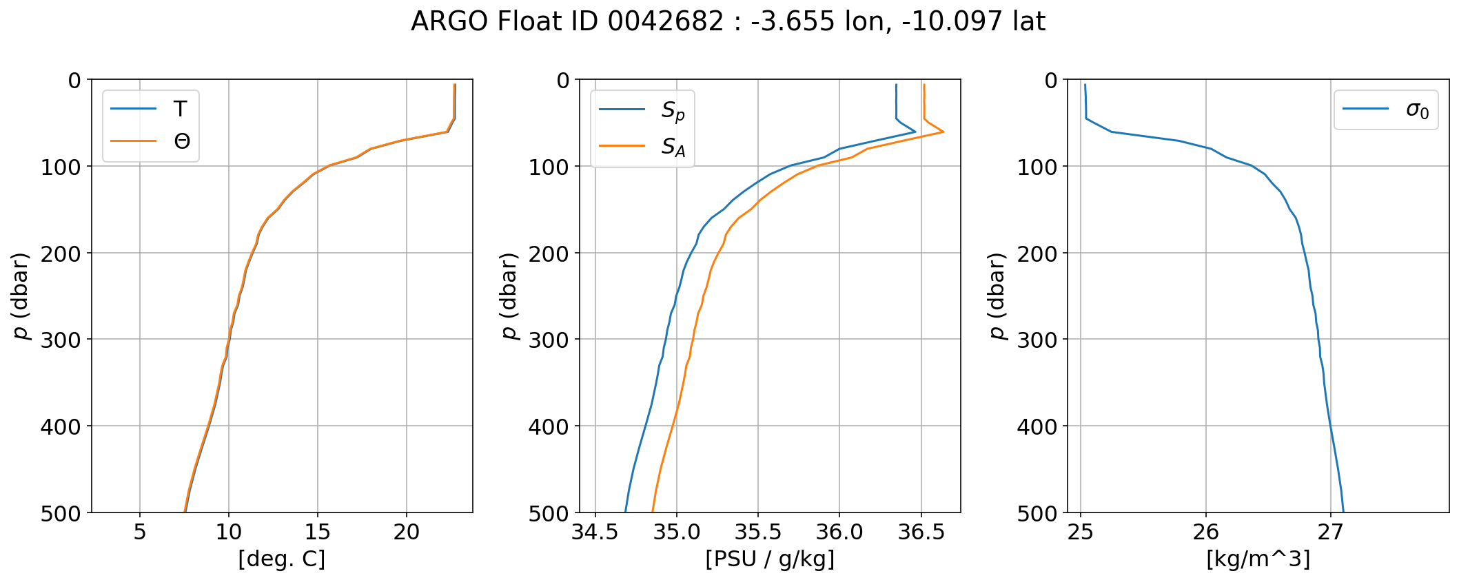
The mixed layer exists primarily because of the winds; the winds generate surface waves which break, and the resulting turbulence homogenizes the properties of the near-surface water.
Generally speaking, the stronger the winds, the deeper the mixed layer. However, buoyancy fluxes can also help determine the mixed layer depth. In winter, strong cooling causes the surface water to become denser than the underlying water. This triggers turbulent convection which deepens the mixed layer.
url = 'http://mixedlayer.ucsd.edu/data/Argo_mixedlayers_monthlyclim_03172021.nc'
file_path = pooch.retrieve(url, known_hash=None)
mld = xr.open_dataset(file_path)
mld = mld.swap_dims({'iLON': 'lon', 'iLAT': 'lat', 'iMONTH': 'month'})
mld
<xarray.Dataset>
Dimensions: (lat: 180, lon: 360, month: 12)
Coordinates:
* lat (lat) float64 -89.5 -88.5 -87.5 -86.5 ... 86.5 87.5 88.5 89.5
* lon (lon) float64 -179.5 -178.5 -177.5 ... 177.5 178.5 179.5
* month (month) float64 1.0 2.0 3.0 4.0 5.0 ... 9.0 10.0 11.0 12.0
Data variables: (12/17)
mld_da_mean (lat, lon, month) float64 ...
mld_dt_mean (lat, lon, month) float64 ...
mld_da_median (lat, lon, month) float64 ...
mld_dt_median (lat, lon, month) float64 ...
mld_da_std (lat, lon, month) float64 ...
mld_dt_std (lat, lon, month) float64 ...
... ...
mlt_dt (lat, lon, month) float64 ...
mls_da (lat, lon, month) float64 ...
mls_dt (lat, lon, month) float64 ...
num (lat, lon, month) float64 ...
longrid (lat, lon) float64 -179.5 -178.5 -177.5 ... 177.5 178.5 179.5
latgrid (lat, lon) float64 -89.5 -89.5 -89.5 -89.5 ... 89.5 89.5 89.5
Attributes:
description: This file was created using \n matlab R2011b with NETCDF Li...
date: [730848.53015047 730848.88790506 730849.28543982 ... 738207...- lat: 180
- lon: 360
- month: 12
- lat(lat)float64-89.5 -88.5 -87.5 ... 88.5 89.5
- long_name :
- Latitude -90 to 90, 1degree
- standard_name :
- latitude
- units :
- degrees
- valid_min :
- -89.5
- valid_max :
- 89.5
- axis :
- Y
- reference_datum :
- geographical coordinates, WGS84 projection
- _CoordinateAxisType :
- Lat
array([-89.5, -88.5, -87.5, -86.5, -85.5, -84.5, -83.5, -82.5, -81.5, -80.5, -79.5, -78.5, -77.5, -76.5, -75.5, -74.5, -73.5, -72.5, -71.5, -70.5, -69.5, -68.5, -67.5, -66.5, -65.5, -64.5, -63.5, -62.5, -61.5, -60.5, -59.5, -58.5, -57.5, -56.5, -55.5, -54.5, -53.5, -52.5, -51.5, -50.5, -49.5, -48.5, -47.5, -46.5, -45.5, -44.5, -43.5, -42.5, -41.5, -40.5, -39.5, -38.5, -37.5, -36.5, -35.5, -34.5, -33.5, -32.5, -31.5, -30.5, -29.5, -28.5, -27.5, -26.5, -25.5, -24.5, -23.5, -22.5, -21.5, -20.5, -19.5, -18.5, -17.5, -16.5, -15.5, -14.5, -13.5, -12.5, -11.5, -10.5, -9.5, -8.5, -7.5, -6.5, -5.5, -4.5, -3.5, -2.5, -1.5, -0.5, 0.5, 1.5, 2.5, 3.5, 4.5, 5.5, 6.5, 7.5, 8.5, 9.5, 10.5, 11.5, 12.5, 13.5, 14.5, 15.5, 16.5, 17.5, 18.5, 19.5, 20.5, 21.5, 22.5, 23.5, 24.5, 25.5, 26.5, 27.5, 28.5, 29.5, 30.5, 31.5, 32.5, 33.5, 34.5, 35.5, 36.5, 37.5, 38.5, 39.5, 40.5, 41.5, 42.5, 43.5, 44.5, 45.5, 46.5, 47.5, 48.5, 49.5, 50.5, 51.5, 52.5, 53.5, 54.5, 55.5, 56.5, 57.5, 58.5, 59.5, 60.5, 61.5, 62.5, 63.5, 64.5, 65.5, 66.5, 67.5, 68.5, 69.5, 70.5, 71.5, 72.5, 73.5, 74.5, 75.5, 76.5, 77.5, 78.5, 79.5, 80.5, 81.5, 82.5, 83.5, 84.5, 85.5, 86.5, 87.5, 88.5, 89.5]) - lon(lon)float64-179.5 -178.5 ... 178.5 179.5
- long_name :
- Longitude -180 to 180, 1degree
- standard_name :
- longitude
- units :
- degrees
- valid_min :
- -179.5
- valid_max :
- 179.5
- axis :
- X
- reference_datum :
- geographical coordinates, WGS84 projection
- _CoordinateAxisType :
- Lon
array([-179.5, -178.5, -177.5, ..., 177.5, 178.5, 179.5])
- month(month)float641.0 2.0 3.0 4.0 ... 10.0 11.0 12.0
- long_name :
- Month
- standard_name :
- Month
- units :
- valid_min :
- 1.0
- valid_max :
- 12.0
- axis :
- reference_datum :
- 1 = January, 12 = December
- _CoordinateAxisType :
- Month
array([ 1., 2., 3., 4., 5., 6., 7., 8., 9., 10., 11., 12.])
- mld_da_mean(lat, lon, month)float64...
- long_name :
- Monthly mean of the MLDs found by the density algorithm in 1 degree bins
- standard_name :
- mld_da_mean
- units :
- meters
- _CoordinateAxis :
- month lat lon
- valid_min :
- 95.0
- valid_max :
- 110.0
- title :
- Monthly mean of the MLDs found by the density algorithm in 1 degree bins
- institution :
- SIO
[777600 values with dtype=float64]
- mld_dt_mean(lat, lon, month)float64...
- long_name :
- Monthly mean of the MLDs found by the density threshold in 1 degree bins
- standard_name :
- mld_dt_mean
- units :
- meters
- _CoordinateAxis :
- month lat lon
- valid_min :
- 95.0
- valid_max :
- 116.0
- title :
- Monthly mean of the MLDs found by the density threshold in 1 degree bins
- institution :
- SIO
[777600 values with dtype=float64]
- mld_da_median(lat, lon, month)float64...
- long_name :
- Monthly median of the MLDs found by the density algorithm in 1 degree bins
- standard_name :
- mld_da_median
- units :
- meters
- _CoordinateAxis :
- month lat lon
- valid_min :
- 95.0
- valid_max :
- 110.0
- title :
- Monthly median of the MLDs found by the density algorithm in 1 degree bins
- institution :
- SIO
[777600 values with dtype=float64]
- mld_dt_median(lat, lon, month)float64...
- long_name :
- Monthly median of the MLDs found by the density threshold in 1 degree bins
- standard_name :
- mld_dt_median
- units :
- meters
- _CoordinateAxis :
- month lat lon
- valid_min :
- 95.0
- valid_max :
- 116.0
- title :
- Monthly median of the MLDs found by the density threshold in 1 degree bins
- institution :
- SIO
[777600 values with dtype=float64]
- mld_da_std(lat, lon, month)float64...
- long_name :
- Monthly standard deviation of the MLDs found by the density algorithm in 1 degree bins
- standard_name :
- mld_da_std
- units :
- meters
- _CoordinateAxis :
- month lat lon
- valid_min :
- 95.0
- valid_max :
- 116.0
- title :
- Monthly standard deviation of the MLDs found by the density algorithm in 1 degree bins
- institution :
- SIO
[777600 values with dtype=float64]
- mld_dt_std(lat, lon, month)float64...
- long_name :
- Monthly standard deviation of the MLDs found by the density threshold in 1 degree bins
- standard_name :
- mld_dt_std
- units :
- meters
- _CoordinateAxis :
- month lat lon
- valid_min :
- 95.0
- valid_max :
- 116.0
- title :
- Monthly standard deviation of the MLDs found by the density threshold in 1 degree bins
- institution :
- SIO
[777600 values with dtype=float64]
- mld_da_max(lat, lon, month)float64...
- long_name :
- Monthly maximum of the MLDs found by the density algorithm in 1 degree bins (average of 3 deepest MLDs)
- standard_name :
- mld_da_max
- units :
- meters
- _CoordinateAxis :
- month lat lon
- valid_min :
- 95.0
- valid_max :
- 120.0
- title :
- Monthly maximum of the MLDs found by the density algorithm in 1 degree bins (average of 3 deepest MLDs)
- institution :
- SIO
[777600 values with dtype=float64]
- mld_dt_max(lat, lon, month)float64...
- long_name :
- Monthly maximum of the MLDs found by the density threshold in 1 degree bins (average of 3 deepest MLDs)
- standard_name :
- mld_dt_max
- units :
- meters
- _CoordinateAxis :
- month lat lon
- valid_min :
- 95.0
- valid_max :
- 120.0
- title :
- Monthly maximum of the MLDs found by the density threshold in 1 degree bins (average of 3 deepest MLDs)
- institution :
- SIO
[777600 values with dtype=float64]
- mlpd_da(lat, lon, month)float64...
- long_name :
- Monthly averages of the ML potential densities found by the density algorithm in 1 degree bins
- standard_name :
- mlpd_da
- units :
- kg/m^3
- _CoordinateAxis :
- month lat lon
- valid_min :
- 95.0
- valid_max :
- 112.0
- title :
- Monthly averages of the ML potential densities found by the density algorithm in 1 degree bins
- institution :
- SIO
[777600 values with dtype=float64]
- mlpd_dt(lat, lon, month)float64...
- long_name :
- Monthly averages of the ML potential densities found by the density threshold in 1 degree bins
- standard_name :
- mlpd_dt
- units :
- kg/m^3
- _CoordinateAxis :
- month lat lon
- valid_min :
- 95.0
- valid_max :
- 116.0
- title :
- Monthly averages of the ML potential densities found by the density threshold in 1 degree bins
- institution :
- SIO
[777600 values with dtype=float64]
- mlt_da(lat, lon, month)float64...
- long_name :
- Monthly averages of the ML conservative temperatures found by the density algorithm in 1 degree bins
- standard_name :
- mlt_da
- units :
- Celsius
- _CoordinateAxis :
- month lat lon
- valid_min :
- 95.0
- valid_max :
- 116.0
- title :
- Monthly averages of the ML conservative temperatures found by the density algorithm in 1 degree bins
- institution :
- SIO
[777600 values with dtype=float64]
- mlt_dt(lat, lon, month)float64...
- long_name :
- Monthly averages of the ML conservative temperatures found by the density threshold in 1 degree bins
- standard_name :
- mlt_dt
- units :
- Celsius
- _CoordinateAxis :
- month lat lon
- valid_min :
- 95.0
- valid_max :
- 116.0
- title :
- Monthly averages of the ML conservative temperatures found by the density threshold in 1 degree bins
- institution :
- SIO
[777600 values with dtype=float64]
- mls_da(lat, lon, month)float64...
- long_name :
- Monthly averages of the ML absolute salinities found by the density algorithm in 1 degree bins
- standard_name :
- mls_da
- units :
- g/kg
- _CoordinateAxis :
- month lat lon
- valid_min :
- 95.0
- valid_max :
- 115.0
- title :
- Monthly averages of the ML absolute salinities found by the density algorithm in 1 degree bins
- institution :
- SIO
[777600 values with dtype=float64]
- mls_dt(lat, lon, month)float64...
- long_name :
- Monthly averages of the ML absolute salinities found by the density threshold in 1 degree bins
- standard_name :
- mls_dt
- units :
- g/kg
- _CoordinateAxis :
- month lat lon
- valid_min :
- 95.0
- valid_max :
- 116.0
- title :
- Monthly averages of the ML absolute salinities found by the density threshold in 1 degree bins
- institution :
- SIO
[777600 values with dtype=float64]
- num(lat, lon, month)float64...
- long_name :
- Number of Argo profiles
- standard_name :
- num
- units :
- _CoordinateAxis :
- month lat lon
- valid_min :
- 109.0
- valid_max :
- 117.0
- title :
- Number of Argo profiles
- institution :
- SIO
[777600 values with dtype=float64]
- longrid(lat, lon)float64...
- long_name :
- Longitude grid
- standard_name :
- longrid
- units :
- Degrees east
- _CoordinateAxis :
- month lat lon
- valid_min :
- 100.0
- valid_max :
- 114.0
- title :
- Longitude grid
- institution :
- SIO
array([[-179.5, -178.5, -177.5, ..., 177.5, 178.5, 179.5], [-179.5, -178.5, -177.5, ..., 177.5, 178.5, 179.5], [-179.5, -178.5, -177.5, ..., 177.5, 178.5, 179.5], ..., [-179.5, -178.5, -177.5, ..., 177.5, 178.5, 179.5], [-179.5, -178.5, -177.5, ..., 177.5, 178.5, 179.5], [-179.5, -178.5, -177.5, ..., 177.5, 178.5, 179.5]]) - latgrid(lat, lon)float64...
- long_name :
- Latitude grid
- standard_name :
- latgrid
- units :
- Degrees north
- _CoordinateAxis :
- month lat lon
- valid_min :
- 97.0
- valid_max :
- 116.0
- title :
- Latitude grid
- institution :
- SIO
array([[-89.5, -89.5, -89.5, ..., -89.5, -89.5, -89.5], [-88.5, -88.5, -88.5, ..., -88.5, -88.5, -88.5], [-87.5, -87.5, -87.5, ..., -87.5, -87.5, -87.5], ..., [ 87.5, 87.5, 87.5, ..., 87.5, 87.5, 87.5], [ 88.5, 88.5, 88.5, ..., 88.5, 88.5, 88.5], [ 89.5, 89.5, 89.5, ..., 89.5, 89.5, 89.5]])
- description :
- This file was created using matlab R2011b with NETCDF Library Functions
- date :
- [730848.53015047 730848.88790506 730849.28543982 ... 738207.42152778 738217.42152778 738227.41736111]
mld.mld_da_max.hvplot('lon', 'lat', clim=(0, 500), label='Maximum Mixed Layer Depth', cmap='Viridis', **opts)
/srv/conda/envs/notebook/lib/python3.8/site-packages/cartopy/io/__init__.py:241: DownloadWarning: Downloading: https://naturalearth.s3.amazonaws.com/110m_physical/ne_110m_land.zip
warnings.warn(f'Downloading: {url}', DownloadWarning)
/srv/conda/envs/notebook/lib/python3.8/site-packages/cartopy/io/__init__.py:241: DownloadWarning: Downloading: https://naturalearth.s3.amazonaws.com/110m_physical/ne_110m_coastline.zip
warnings.warn(f'Downloading: {url}', DownloadWarning)
Simple 1D Model
The mixed layer is the part of the ocean that is in direct contact with the atmosphere, and so our equations for air-sea interaction are equations for the evolution of the mixed layer. For the sake of simplicity, we will begin by considering just a one-dimensional model, where all exchange is in the vertical. (In other words, we will not consider lateral exchanges of heat and salt within the mixed layer.) Furthermore, we will assume that the mixed layer is totally isolated from the thermocline and does not exchange heat and salt with the water below. Both these assumptions are unrealistic, but they are a useful starting point.
In this model, the mixed layer thermodynamic state is characterized by three fundamental state variables: \(\Theta\) (conservative temperature), \(S_A\) (absolute salinity), and \(h\), the mixed layer depth. Through the equation of state, \(\Theta\) and \(S_A\) determine the mixed layer potential density. (The pressure is irrelevant for now, but in this 1D model, it is simply proportional to depth.) We now describe how air-sea exchange influences the evolution of \(\Theta\) and \(S_A\).
Heat Exchange
The heat content of the mixed layer (per unit area) is given by.
If the mixed layer is isolated from the interior, the first law of thermodynamics can be written as
where \(Q\) is the air-to-sea heat flux.
Because density \(\rho\) only changes by a about 0.1% during air-sea interaction, it is reasonable to approximate \(\rho \simeq \rho_0\). If we further assume that the mixed layer depth \(h\) doesn’t change, we can write the heat equation as
Components of the Heat Flux
We divide the heat flux \(Q\) into four separate components associated with different physical processes.
registry = {
"hfns11a.nc.Z": None,
"hfls11a.nc.Z": None,
"hfss11a.nc.Z": None,
"rss11a.nc.Z": None,
"rls11a.nc.Z": None
}
POOCH = pooch.create(
path=pooch.os_cache("Grist_Josey_2003"),
base_url="ftp://ftp.noc.soton.ac.uk/pub/sxj/clim/netcdf/",
registry=registry
)
fnames = {fname: POOCH.fetch(fname) for fname in registry}
import unlzw3
def uncompress(input_fname):
assert input_fname[-2:] == '.Z'
output_fname = input_fname[:-2]
with open(input_fname, "rb") as fp:
uncompressed_data = unlzw3.unlzw(fp.read())
with open(output_fname, "wb") as fp:
fp.write(uncompressed_data)
return output_fname
fnames_uncompressed = [uncompress(f) for f in fnames.values()]
noca = xr.open_mfdataset(fnames_uncompressed, combine='by_coords')
noca = noca.assign_coords({'month': noca.time.dt.month}).swap_dims({'time': 'month'})
noca
/srv/conda/envs/notebook/lib/python3.8/site-packages/xarray/coding/times.py:119: SerializationWarning: Ambiguous reference date string: 2-1-1 0. The first value is assumed to be the year hence will be padded with zeros to remove the ambiguity (the padded reference date string is: 0002-1-1 0). To remove this message, remove the ambiguity by padding your reference date strings with zeros.
warnings.warn(warning_msg, SerializationWarning)
/srv/conda/envs/notebook/lib/python3.8/site-packages/xarray/coding/times.py:527: SerializationWarning: Unable to decode time axis into full numpy.datetime64 objects, continuing using cftime.datetime objects instead, reason: dates out of range
dtype = _decode_cf_datetime_dtype(data, units, calendar, self.use_cftime)
/srv/conda/envs/notebook/lib/python3.8/site-packages/xarray/core/indexing.py:572: SerializationWarning: Unable to decode time axis into full numpy.datetime64 objects, continuing using cftime.datetime objects instead, reason: dates out of range
return np.asarray(array[self.key], dtype=None)
<xarray.Dataset>
Dimensions: (latitude: 170, longitude: 360, month: 12)
Coordinates:
time (month) object 0002-01-01 00:00:00 ... 0002-12-01 00:00:00
* longitude (longitude) float64 -179.5 -178.5 -177.5 ... 177.5 178.5 179.5
* latitude (latitude) float64 -84.5 -83.5 -82.5 -81.5 ... 82.5 83.5 84.5
* month (month) int64 1 2 3 4 5 6 7 8 9 10 11 12
Data variables:
hfls11a (month, latitude, longitude) float32 dask.array<chunksize=(12, 170, 360), meta=np.ndarray>
hfns11a (month, latitude, longitude) float32 dask.array<chunksize=(12, 170, 360), meta=np.ndarray>
hfss11a (month, latitude, longitude) float32 dask.array<chunksize=(12, 170, 360), meta=np.ndarray>
rls11a (month, latitude, longitude) float32 dask.array<chunksize=(12, 170, 360), meta=np.ndarray>
rss11a (month, latitude, longitude) float32 dask.array<chunksize=(12, 170, 360), meta=np.ndarray>
Attributes:
Conventions: COARDS
calendar: standard
comments: Climatological estimate based on ship meteorological report...
model:
center: National Oceanography Centre, Southampton, UK- latitude: 170
- longitude: 360
- month: 12
- time(month)object0002-01-01 00:00:00 ... 0002-12-...
array([cftime.DatetimeGregorian(2, 1, 1, 0, 0, 0, 0, has_year_zero=False), cftime.DatetimeGregorian(2, 2, 1, 0, 0, 0, 0, has_year_zero=False), cftime.DatetimeGregorian(2, 3, 1, 0, 0, 0, 0, has_year_zero=False), cftime.DatetimeGregorian(2, 4, 1, 0, 0, 0, 0, has_year_zero=False), cftime.DatetimeGregorian(2, 5, 1, 0, 0, 0, 0, has_year_zero=False), cftime.DatetimeGregorian(2, 6, 1, 0, 0, 0, 0, has_year_zero=False), cftime.DatetimeGregorian(2, 7, 1, 0, 0, 0, 0, has_year_zero=False), cftime.DatetimeGregorian(2, 8, 1, 0, 0, 0, 0, has_year_zero=False), cftime.DatetimeGregorian(2, 9, 1, 0, 0, 0, 0, has_year_zero=False), cftime.DatetimeGregorian(2, 10, 1, 0, 0, 0, 0, has_year_zero=False), cftime.DatetimeGregorian(2, 11, 1, 0, 0, 0, 0, has_year_zero=False), cftime.DatetimeGregorian(2, 12, 1, 0, 0, 0, 0, has_year_zero=False)], dtype=object) - longitude(longitude)float64-179.5 -178.5 ... 178.5 179.5
- units :
- degrees_east
- long_name :
- Longitude
array([-179.5, -178.5, -177.5, ..., 177.5, 178.5, 179.5])
- latitude(latitude)float64-84.5 -83.5 -82.5 ... 83.5 84.5
- units :
- degrees_north
- long_name :
- Latitude
array([-84.5, -83.5, -82.5, -81.5, -80.5, -79.5, -78.5, -77.5, -76.5, -75.5, -74.5, -73.5, -72.5, -71.5, -70.5, -69.5, -68.5, -67.5, -66.5, -65.5, -64.5, -63.5, -62.5, -61.5, -60.5, -59.5, -58.5, -57.5, -56.5, -55.5, -54.5, -53.5, -52.5, -51.5, -50.5, -49.5, -48.5, -47.5, -46.5, -45.5, -44.5, -43.5, -42.5, -41.5, -40.5, -39.5, -38.5, -37.5, -36.5, -35.5, -34.5, -33.5, -32.5, -31.5, -30.5, -29.5, -28.5, -27.5, -26.5, -25.5, -24.5, -23.5, -22.5, -21.5, -20.5, -19.5, -18.5, -17.5, -16.5, -15.5, -14.5, -13.5, -12.5, -11.5, -10.5, -9.5, -8.5, -7.5, -6.5, -5.5, -4.5, -3.5, -2.5, -1.5, -0.5, 0.5, 1.5, 2.5, 3.5, 4.5, 5.5, 6.5, 7.5, 8.5, 9.5, 10.5, 11.5, 12.5, 13.5, 14.5, 15.5, 16.5, 17.5, 18.5, 19.5, 20.5, 21.5, 22.5, 23.5, 24.5, 25.5, 26.5, 27.5, 28.5, 29.5, 30.5, 31.5, 32.5, 33.5, 34.5, 35.5, 36.5, 37.5, 38.5, 39.5, 40.5, 41.5, 42.5, 43.5, 44.5, 45.5, 46.5, 47.5, 48.5, 49.5, 50.5, 51.5, 52.5, 53.5, 54.5, 55.5, 56.5, 57.5, 58.5, 59.5, 60.5, 61.5, 62.5, 63.5, 64.5, 65.5, 66.5, 67.5, 68.5, 69.5, 70.5, 71.5, 72.5, 73.5, 74.5, 75.5, 76.5, 77.5, 78.5, 79.5, 80.5, 81.5, 82.5, 83.5, 84.5]) - month(month)int641 2 3 4 5 6 7 8 9 10 11 12
array([ 1, 2, 3, 4, 5, 6, 7, 8, 9, 10, 11, 12])
- hfls11a(month, latitude, longitude)float32dask.array<chunksize=(12, 170, 360), meta=np.ndarray>
- comments :
- Inverse analysis estimate, Grist and Josey (2003)
- long_name :
- Heat flux latent surface (Positive for heat gain by the ocean)
- units :
- W/m^2
- grid_name :
- generic grid
- grid_type :
- generic
- level_description :
- Earth surface
- time_statistic :
- average
Array Chunk Bytes 2.80 MiB 2.80 MiB Shape (12, 170, 360) (12, 170, 360) Count 2 Tasks 1 Chunks Type float32 numpy.ndarray - hfns11a(month, latitude, longitude)float32dask.array<chunksize=(12, 170, 360), meta=np.ndarray>
- comments :
- Inverse analysis estimate, Grist and Josey (2003)
- long_name :
- Heat flux net surface (Positive for heat gain by the ocean)
- units :
- W/m^2
- grid_name :
- generic grid
- grid_type :
- generic
- level_description :
- Earth surface
- time_statistic :
- average
Array Chunk Bytes 2.80 MiB 2.80 MiB Shape (12, 170, 360) (12, 170, 360) Count 2 Tasks 1 Chunks Type float32 numpy.ndarray - hfss11a(month, latitude, longitude)float32dask.array<chunksize=(12, 170, 360), meta=np.ndarray>
- comments :
- Inverse analysis estimate, Grist and Josey (2003)
- long_name :
- Heat flux sensible surface (Positive for heat gain by the ocean)
- units :
- W/m^2
- grid_name :
- generic grid
- grid_type :
- generic
- level_description :
- Earth surface
- time_statistic :
- average
Array Chunk Bytes 2.80 MiB 2.80 MiB Shape (12, 170, 360) (12, 170, 360) Count 2 Tasks 1 Chunks Type float32 numpy.ndarray - rls11a(month, latitude, longitude)float32dask.array<chunksize=(12, 170, 360), meta=np.ndarray>
- comments :
- Inverse analysis estimate, Grist and Josey (2003)
- long_name :
- Heat flux net longwave surface (Positive for heat gain by the ocean)
- units :
- W/m^2
- grid_name :
- generic grid
- grid_type :
- generic
- level_description :
- Earth surface
- time_statistic :
- average
Array Chunk Bytes 2.80 MiB 2.80 MiB Shape (12, 170, 360) (12, 170, 360) Count 2 Tasks 1 Chunks Type float32 numpy.ndarray - rss11a(month, latitude, longitude)float32dask.array<chunksize=(12, 170, 360), meta=np.ndarray>
- comments :
- Inverse analysis estimate, Grist and Josey (2003)
- long_name :
- Heat flux net shortwave surface (Positive for heat gain by the ocean)
- units :
- W/m^2
- grid_name :
- generic grid
- grid_type :
- generic
- level_description :
- Earth surface
- time_statistic :
- average
Array Chunk Bytes 2.80 MiB 2.80 MiB Shape (12, 170, 360) (12, 170, 360) Count 2 Tasks 1 Chunks Type float32 numpy.ndarray
- Conventions :
- COARDS
- calendar :
- standard
- comments :
- Climatological estimate based on ship meteorological reports and adjusted using inverse analysis: National Oceanography Centre surface flux climatology Version 1.1a (NOC1.1a). See README file for full details. Contact: Simon.A.Josey@noc.soton.ac.uk.
- model :
- center :
- National Oceanography Centre, Southampton, UK
Radiative Fluxes
The radiative fluxes in the earth system are often partitioned into a shortwave and longwave component. These names refer to the wavelength of the electromagnetic waves which constitute the radiation. These components occupy very distinct parts of the electromagnetic spectrum. Radiation emitted from the sun is shortwave radiation, while radiation emitted from the earth itself is longwave radiation. The dramatic difference in wavelengths emitted from each body is a result of Planck’s law of blackbody radiation, which describes how the emission wavelength depends on temperature. Solar radiation has a shorter wavelength than terrestrial because the sun is much hotter than the earth.
Image(url="https://upload.wikimedia.org/wikipedia/commons/7/7c/Atmospheric_Transmission.png")
Atmospheric Transmission. Licensed CC BY-SA 3.0 Creative Commons Attribution-Share Alike 3.0
Image(url="https://upload.wikimedia.org/wikipedia/commons/b/bb/"
"The-NASA-Earth%27s-Energy-Budget-Poster-Radiant-Energy-System-satellite-infrared-radiation-fluxes.jpg")

By NASA, Public domain. Via Wikimedia Commons
Shortwave Radiation
The average value of incoming solar radiation at the top of Earth’s atmosphere is 342 W m\(^{-2}\), although this value varies considerably with latitude and season. Some of the solar radiation is absorbed by the atmosphere or reflected back to space by clouds and aerosols, never reaching the ocean. Furthermore, the ocean doesn’t absorb all of the shortwave radiation that reaches its surface; some is also reflected back to space. The albedo \(\alpha\) describes how much radiation is absorbed versus reflected. Therefore, the shortwave heating is given by
where \(Q^{inc}_{sw}\) is the incident shortwave radiation.
Albedo
An albedo of 0 means that all of the incident radiation is absorbed. The ocean’s average albedo is about 0.06, although it does vary somewhat depending on sea state. This relatively low albedo means that the ocean is a very effective absorber of radiation, especially compared to ice. The strong change in albedo that occurs when the high-latitude ocean freezes is melts is therefore a significant climate feedback.
Image(url='https://upload.wikimedia.org/wikipedia/commons/e/e2/Ceres_2004_clear_sky_albedo.png', width=800)
By Giorgiogp2 (Own work). License CC BY-SA 3.0 or GFDL, via Wikimedia Commons
noca.rss11a.hvplot('longitude', 'latitude', clim=(-300, 300), label=noca.rss11a.long_name, cmap='RdBu_r', **opts)
df_zm = noca.fillna(0.).mean(dim=('month', 'longitude')).to_dataframe()
new_columns = {v: re.sub(r'Heat flux (.*) surface \(.*', r'\1', noca[v].long_name) for v in noca.data_vars}
df_zm = df_zm.rename(columns=new_columns)
df_zm.head()
| latent | net | sensible | net longwave | net shortwave | |
|---|---|---|---|---|---|
| latitude | |||||
| -84.5 | 0.0 | 0.0 | 0.0 | 0.0 | 0.0 |
| -83.5 | 0.0 | 0.0 | 0.0 | 0.0 | 0.0 |
| -82.5 | 0.0 | 0.0 | 0.0 | 0.0 | 0.0 |
| -81.5 | 0.0 | 0.0 | 0.0 | 0.0 | 0.0 |
| -80.5 | 0.0 | 0.0 | 0.0 | 0.0 | 0.0 |
df_zm.hvplot.line(x='latitude', y='net shortwave', line_width=4, grid=True, legend='top')
Longwave Radiation
Because of its much lower temperature, the earth emits radiation in the longwave (i.e. infrared) band. On a global scale, emission is the main way the planet balances the incoming solar radiation to maintain its thermal equilibrium. The power of emitted radiation is strongly dependent on temperature; specifically, the Stefan-Boltzman law states that
where \(\sigma = 5.67 \times 10^-8\) W m\(^{-2}\) K\(^{-4}\) is the Stefan-Boltzman constant. (It is important to remember to use absolute temperature in deg. Kelvin when evaluating this formula.) Here we have chosen to maintain the same sign convention for longwave radiation as for shortwave.
\(Q_{lw}^{emitted}\) is not the only contribution to the longwave flux. The atmosphere also emits longwave radiation itself, and some of this radiation is absorbed by the ocean. There is a large amount of cancellation between these two components, but in the net The fact that \(Q_{lw}\) is negative definite means that longwave emissions acts to cool the ocean.
Longwave cooling is indeed a significant sink of heat from the ocean. The mean value of the longwave cooling is around -50 W m\(^{-2}\).
noca.rls11a.hvplot('longitude', 'latitude', clim=(-100, 100), label=noca.rls11a.long_name, cmap='RdBu_r', **opts)
df_zm.hvplot.line(x='latitude', y=['net shortwave', 'net longwave'], line_width=4, grid=True, legend='top', height=400)
Sensible Heat Flux
Radiative fluxes transmit heat energy over long distances, e.g.~from the sun to the earth. Sensible heat exchange instead depends on direct molecular contact between air and water. The molecules of the two fluids bump against each other, thereby exchanging heat energy. When the ocean and air temperature are the same, the sensible heat flux is therefore zero. When they differ, heat is exchanged in such as way as to homogenize the temperature. This is analogous to the phenomenon of “Newtonian cooling’’ commonly studied in introductory physics courses.
The rate of exchange is highly dependent on the sea state, and in particular on the winds, which generate breaking waves and turbulence. It is easy to imagine how breaking waves enhance the exchange of heat: they literally pull air down into the water (bubbles) and splash water up into the air (sea spray). It is much harder to quantify this process mathematically. Nevertheless, laboratory experiments and field campaigns have permitted us to develop empirical formulas to do so.
Bulk Formula
The commonly accepted formula for sensible heat flux is
The subscript \(_{10}\) refers to the properties of air at 10 m altitude (\(T_{10}\) is air temperature at 10 m). Although this height is somewhat arbitrary, it is a widely-used convention. \(\Delta \mathbf{u} = \mathbf{u}_{10} - \mathbf{u}\) refers to the difference between the wind speed at 10 m and the ocean current speed. \(c_p^{air} = 1030\) J kg\(^{-1}\) K\(^{-1}\) is the specific heat of air and \(\rho^{air}\) is the density of air (approximately \(1.3\) kg m\(^{-3}\)). Note it is the in-situ temperature \(T\), not conservative temperature, which appears in the bulk formula.
Drag Coefficient
All of the complexity and difficulty of turbulent air-sea exchange is absorbed into the parameter \(C_H\), the turbulent transfer coefficient for sensible heat exchange. This non-dimensional coefficient is \(O(1000)\) but is a strongly nonlinear function of \(|\Delta \mathbf{u}|\). It also depends on the stability of the stratification within the atmospheric boundary layer. The figure below illustrates this dependence.
Image(filename='04_images/LY09_Drag_Coefficient.png', width=800)
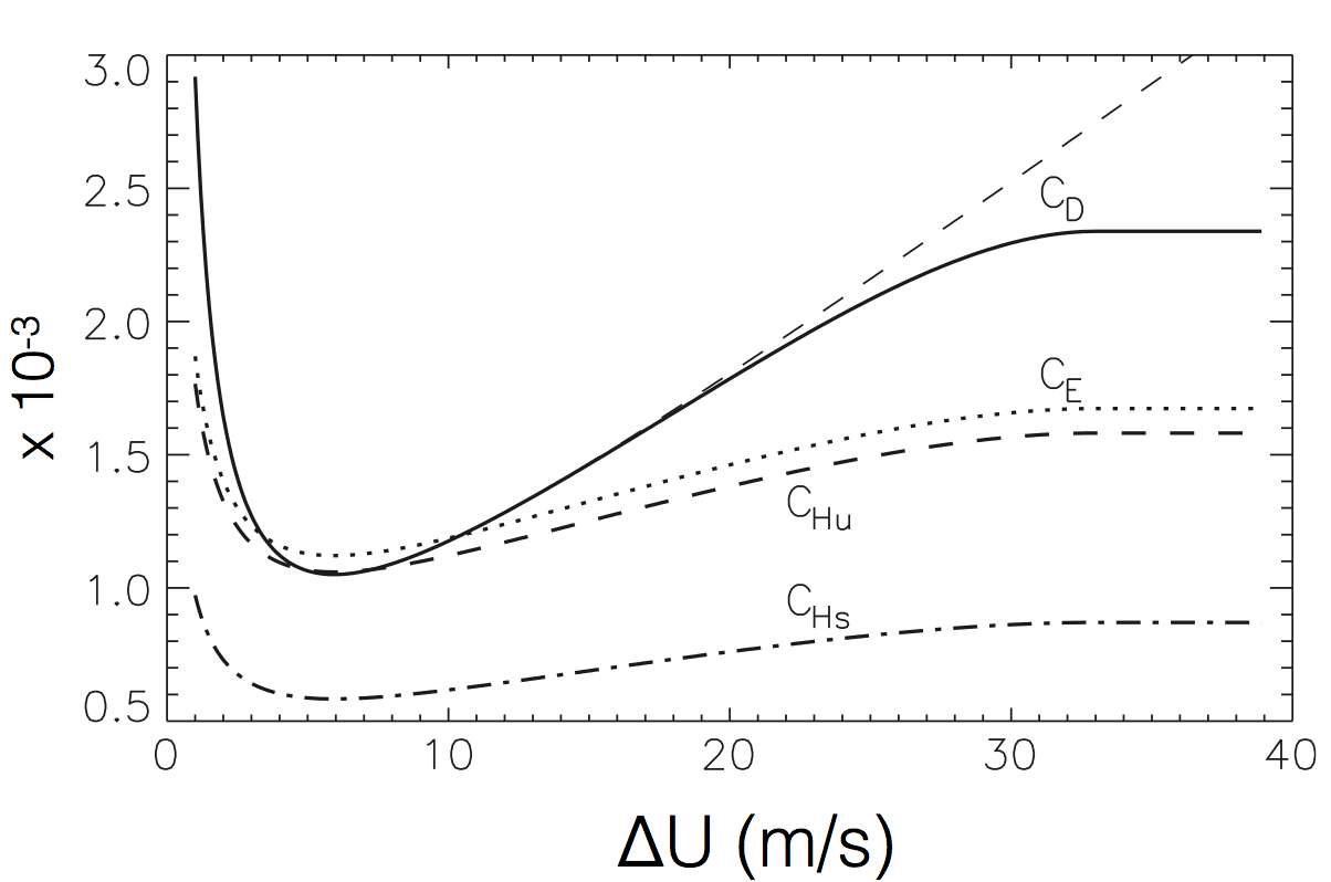
Turbulent transfer coefficients as a function of wind speed, taken from Large and Yeager (2009). Note that \(C_H\) is different in stable, (\(C_{H_s}\)) and unstable (\(C_{H_u}\)) atmospheric stratification.
For strong winds, \(C_H\) is a positive function of \(|\Delta \mathbf{u}|\). But as \( | \Delta \mathbf{u} | \) approaches zero, \(C_H\) actually increases very rapidly. This means that the heat exchange doesn’t necessarily vanish for very weak winds, as one might mistakenly conclude from the figure. Further refining our description of \(C_H\), especially for extremely strong winds (i.e.~within hurricanes) is an ongoing topic of study for air-sea-interaction researchers.
noca.hfss11a.hvplot('longitude', 'latitude', clim=(-100, 100), label=noca.hfss11a.long_name, cmap='RdBu_r', **opts)
df_zm.hvplot.line(x='latitude', y=['net shortwave', 'net longwave', 'sensible'], line_width=4, grid=True, legend='top', height=400)
The annual mean contribution of \(Q_s\) to \(Q\) is almost negligible. This is because, on average, the \(T\) and \(T_{10}\) are very close. There is, however, a strong seasonal cycle in sensible heat exchange. Because of the large ocean heat capacity, the ocean is usually colder than the air in summer and warmer than the air in the winter. This drives important seasonal changes in circulation.
Latent Heat Flux
The latent heat flux is produced when seawater evaporates to become atmospheric water vapor. This process requires thermodynamic energy and therefore extracts heat from the ocean. The latent heat flux is given by
where \(E\) is the evaporation rate (in kg m\(^{-2}\) s\(^{-1}\)), and \(L_e \simeq 2.5 \times 10^6\) J kg\(^{-1}\) is the latent heat of vaporization. The fact that \(Q_{lh}\) is negative is due to our sign convention: the latent heat flux always cools the ocean
Evaporation Rate
What sets the evaporation rate \(E\)? As with sensible heat, evaporation is a turbulent exchange which depends on direct molecular contact between air and water. It is given by another bulk formula:
where \(q_{10}\) and \(q_{sat}\) refer, respectively, to the specific humidity of the air at 10 m and the saturation specific humidity right at the sea surface, and \(c_E\) is the exchange coefficient for water vapor. Specific humidity measures the mass fraction of water vapor in air. It is a non-dimensional unit but is frequently reported as g kg\(^{-1}\) (grams of water per kilogram of air).
Saturation Specific Humidty
The maximum amount of water vapor that it can hold is called the saturation specific humidity. This quantity is an exponential function of the air temperature. The relationship between \(q_{sat}\) and temperature is given by the Clausius-Clapeyron relation. A practical formula for evaluating the Clausius-Clapeyron relation over the ocean is
Right at the sea-surface, the air is always at the same temperature as the ocean (\(T\)) and is always completely saturated; that’s why \(q_{sat}\) is a function of SST. But at 10 m altitude, the air can have a different specific humidity due to atmospheric circulation. If the two values of \(q\) are not equal, the ocean will evaporate at rate \(E\).
noca.hfls11a.hvplot('longitude', 'latitude', clim=(-200, 200), label=noca.hfls11a.long_name, cmap='RdBu_r', **opts)
\(Q_{lh}\) is the dominant mechanism for cooling the ocean, with an global, annual mean value of close to 100 W m\(^{-2}\). \(Q_{lh}\) is strongest where strong, dry continental winds blow over the oceans, as occurs near the western boundaries of the midlatitude basins (e.g. over the Gulf Stream).
Net Air Sea Flux
(df_zm.hvplot.line(x='latitude', y=['net shortwave', 'net longwave', 'sensible', 'latent'], line_width=4, grid=True, legend='top', height=400)
* df_zm.hvplot.line(x='latitude', y='net', color='black', label='net', legend=True, line_width=6))
Looking at all the fluxes together, we see that there is strong compensation between shortwave heating and the other processes, which primarily cool the ocean in a mean sense.
The general pattern is net heat gain in the topics and net heat loss near the poles. To keep the ocean in a steady state, ocean circulation must therefore transport heat from equator to pole. There are also important hemispheric aysmmetries: the high-latitude Southern Ocean has regions of significant net heat gain.
noca.hfns11a.mean(dim='month').hvplot('longitude', 'latitude', clim=(-200, 200), label=('Annual Mean' + noca.hfns11a.long_name), cmap='RdBu_r', **opts)
/srv/conda/envs/notebook/lib/python3.8/site-packages/dask/array/numpy_compat.py:40: RuntimeWarning: invalid value encountered in true_divide
x = np.divide(x1, x2, out)
Freshwater Fluxes
We have already talked about evaporation in the context of latent heat fluxes. More generally, the ocean exchanges water with the atmosphere via evaporation, precipitation, and runoff. These fluxes have a rather negligible impact on the ocean volume, but they have a very strong impact on salinity.
Image(url="https://upload.wikimedia.org/wikipedia/commons/thumb/b/b1/"
'Diagram_of_the_Water_Cycle.jpg/1024px-Diagram_of_the_Water_Cycle.jpg')

By Ehud Tal (Own work) CC BY-SA 4.0, via Wikimedia Commons https://commons.wikimedia.org/wiki/File:Diagram_of_the_Water_Cycle.jpg
evap = xr.open_dataset('http://kage.ldeo.columbia.edu:81/expert/home/.OTHER/.richard/.whoi/.oaflux/.data_v3/.monthly/.evaporation/.evapr.nc/dods', decode_times=False)
evap.T.attrs['calendar'] = '360_day'
evap = xr.decode_cf(evap)
evap.load()
<xarray.Dataset>
Dimensions: (T: 688, lat: 180, lon: 360)
Coordinates:
* T (T) object 1958-01-16 00:00:00 ... 2015-04-16 00:00:00
* lat (lat) float32 -89.5 -88.5 -87.5 -86.5 -85.5 ... 86.5 87.5 88.5 89.5
* lon (lon) float32 0.5 1.5 2.5 3.5 4.5 ... 355.5 356.5 357.5 358.5 359.5
Data variables:
evapr (T, lat, lon) float32 nan nan nan nan nan ... nan nan nan nan nan
Attributes:
nco_openmp_thread_number: 1
Conventions: IRIDL
history: Tue Jul 21 15:45:00 2015: ncatted -a gridtype,...
NCO: 4.3.7- T: 688
- lat: 180
- lon: 360
- T(T)object1958-01-16 00:00:00 ... 2015-04-...
- pointwidth :
- 1.0
- gridtype :
- 0
array([cftime.Datetime360Day(1958, 1, 16, 0, 0, 0, 0, has_year_zero=False), cftime.Datetime360Day(1958, 2, 16, 0, 0, 0, 0, has_year_zero=False), cftime.Datetime360Day(1958, 3, 16, 0, 0, 0, 0, has_year_zero=False), ..., cftime.Datetime360Day(2015, 2, 16, 0, 0, 0, 0, has_year_zero=False), cftime.Datetime360Day(2015, 3, 16, 0, 0, 0, 0, has_year_zero=False), cftime.Datetime360Day(2015, 4, 16, 0, 0, 0, 0, has_year_zero=False)], dtype=object) - lat(lat)float32-89.5 -88.5 -87.5 ... 88.5 89.5
- pointwidth :
- 1.0
- range :
- 89.5S to 89.5N
- long_name :
- latitude
- gridtype :
- 0
- units :
- degree_north
array([-89.5, -88.5, -87.5, -86.5, -85.5, -84.5, -83.5, -82.5, -81.5, -80.5, -79.5, -78.5, -77.5, -76.5, -75.5, -74.5, -73.5, -72.5, -71.5, -70.5, -69.5, -68.5, -67.5, -66.5, -65.5, -64.5, -63.5, -62.5, -61.5, -60.5, -59.5, -58.5, -57.5, -56.5, -55.5, -54.5, -53.5, -52.5, -51.5, -50.5, -49.5, -48.5, -47.5, -46.5, -45.5, -44.5, -43.5, -42.5, -41.5, -40.5, -39.5, -38.5, -37.5, -36.5, -35.5, -34.5, -33.5, -32.5, -31.5, -30.5, -29.5, -28.5, -27.5, -26.5, -25.5, -24.5, -23.5, -22.5, -21.5, -20.5, -19.5, -18.5, -17.5, -16.5, -15.5, -14.5, -13.5, -12.5, -11.5, -10.5, -9.5, -8.5, -7.5, -6.5, -5.5, -4.5, -3.5, -2.5, -1.5, -0.5, 0.5, 1.5, 2.5, 3.5, 4.5, 5.5, 6.5, 7.5, 8.5, 9.5, 10.5, 11.5, 12.5, 13.5, 14.5, 15.5, 16.5, 17.5, 18.5, 19.5, 20.5, 21.5, 22.5, 23.5, 24.5, 25.5, 26.5, 27.5, 28.5, 29.5, 30.5, 31.5, 32.5, 33.5, 34.5, 35.5, 36.5, 37.5, 38.5, 39.5, 40.5, 41.5, 42.5, 43.5, 44.5, 45.5, 46.5, 47.5, 48.5, 49.5, 50.5, 51.5, 52.5, 53.5, 54.5, 55.5, 56.5, 57.5, 58.5, 59.5, 60.5, 61.5, 62.5, 63.5, 64.5, 65.5, 66.5, 67.5, 68.5, 69.5, 70.5, 71.5, 72.5, 73.5, 74.5, 75.5, 76.5, 77.5, 78.5, 79.5, 80.5, 81.5, 82.5, 83.5, 84.5, 85.5, 86.5, 87.5, 88.5, 89.5], dtype=float32) - lon(lon)float320.5 1.5 2.5 ... 357.5 358.5 359.5
- pointwidth :
- 1.0
- range :
- 0.5 to 359.5
- long_name :
- longitude
- modulus :
- 360.0
- gridtype :
- 1
- units :
- degree_east
array([ 0.5, 1.5, 2.5, ..., 357.5, 358.5, 359.5], dtype=float32)
- evapr(T, lat, lon)float32nan nan nan nan ... nan nan nan nan
- units :
- cm/yr
- valid_max :
- 3276.7
- comments :
- monthly mean evaporation rate
- valid_min :
- -3276.8
array([[[nan, nan, nan, ..., nan, nan, nan], [nan, nan, nan, ..., nan, nan, nan], [nan, nan, nan, ..., nan, nan, nan], ..., [nan, nan, nan, ..., nan, nan, nan], [nan, nan, nan, ..., nan, nan, nan], [nan, nan, nan, ..., nan, nan, nan]], [[nan, nan, nan, ..., nan, nan, nan], [nan, nan, nan, ..., nan, nan, nan], [nan, nan, nan, ..., nan, nan, nan], ..., [nan, nan, nan, ..., nan, nan, nan], [nan, nan, nan, ..., nan, nan, nan], [nan, nan, nan, ..., nan, nan, nan]], [[nan, nan, nan, ..., nan, nan, nan], [nan, nan, nan, ..., nan, nan, nan], [nan, nan, nan, ..., nan, nan, nan], ..., ... ..., [nan, nan, nan, ..., nan, nan, nan], [nan, nan, nan, ..., nan, nan, nan], [nan, nan, nan, ..., nan, nan, nan]], [[nan, nan, nan, ..., nan, nan, nan], [nan, nan, nan, ..., nan, nan, nan], [nan, nan, nan, ..., nan, nan, nan], ..., [nan, nan, nan, ..., nan, nan, nan], [nan, nan, nan, ..., nan, nan, nan], [nan, nan, nan, ..., nan, nan, nan]], [[nan, nan, nan, ..., nan, nan, nan], [nan, nan, nan, ..., nan, nan, nan], [nan, nan, nan, ..., nan, nan, nan], ..., [nan, nan, nan, ..., nan, nan, nan], [nan, nan, nan, ..., nan, nan, nan], [nan, nan, nan, ..., nan, nan, nan]]], dtype=float32)
- nco_openmp_thread_number :
- 1
- Conventions :
- IRIDL
- history :
- Tue Jul 21 15:45:00 2015: ncatted -a gridtype,lon,o,d,1 evapr.nc Tue Jul 21 15:44:09 2015: ncatted -a units,lat,o,c,degree_north evapr.nc Tue Jul 21 15:44:00 2015: ncatted -a units,lon,o,c,degree_east evapr.nc Tue Jul 21 10:44:26 2015: ncks --mk_rec_dmn T temp/evapr.nc temp/evapr-1958.nc
- NCO :
- 4.3.7
precip = xr.open_dataset('http://iridl.ldeo.columbia.edu/SOURCES/.NASA/.GPCP/.V2p1/.multi-satellite/.prcp/dods', decode_times=False)
precip.T.attrs['calendar'] = '360_day'
precip = xr.decode_cf(precip)
precip.load()
<xarray.Dataset>
Dimensions: (T: 363, X: 144, Y: 72)
Coordinates:
* X (X) float32 1.25 3.75 6.25 8.75 11.25 ... 351.2 353.8 356.2 358.8
* T (T) object 1979-01-16 00:00:00 ... 2009-03-16 00:00:00
* Y (Y) float32 88.75 86.25 83.75 81.25 ... -81.25 -83.75 -86.25 -88.75
Data variables:
prcp (T, Y, X) float32 nan nan nan nan ... 0.1052 0.1064 0.1063 0.1062
Attributes:
Conventions: IRIDL- T: 363
- X: 144
- Y: 72
- X(X)float321.25 3.75 6.25 ... 356.2 358.8
- standard_name :
- longitude
- pointwidth :
- 2.5
- gridtype :
- 1
- units :
- degree_east
array([ 1.25, 3.75, 6.25, 8.75, 11.25, 13.75, 16.25, 18.75, 21.25, 23.75, 26.25, 28.75, 31.25, 33.75, 36.25, 38.75, 41.25, 43.75, 46.25, 48.75, 51.25, 53.75, 56.25, 58.75, 61.25, 63.75, 66.25, 68.75, 71.25, 73.75, 76.25, 78.75, 81.25, 83.75, 86.25, 88.75, 91.25, 93.75, 96.25, 98.75, 101.25, 103.75, 106.25, 108.75, 111.25, 113.75, 116.25, 118.75, 121.25, 123.75, 126.25, 128.75, 131.25, 133.75, 136.25, 138.75, 141.25, 143.75, 146.25, 148.75, 151.25, 153.75, 156.25, 158.75, 161.25, 163.75, 166.25, 168.75, 171.25, 173.75, 176.25, 178.75, 181.25, 183.75, 186.25, 188.75, 191.25, 193.75, 196.25, 198.75, 201.25, 203.75, 206.25, 208.75, 211.25, 213.75, 216.25, 218.75, 221.25, 223.75, 226.25, 228.75, 231.25, 233.75, 236.25, 238.75, 241.25, 243.75, 246.25, 248.75, 251.25, 253.75, 256.25, 258.75, 261.25, 263.75, 266.25, 268.75, 271.25, 273.75, 276.25, 278.75, 281.25, 283.75, 286.25, 288.75, 291.25, 293.75, 296.25, 298.75, 301.25, 303.75, 306.25, 308.75, 311.25, 313.75, 316.25, 318.75, 321.25, 323.75, 326.25, 328.75, 331.25, 333.75, 336.25, 338.75, 341.25, 343.75, 346.25, 348.75, 351.25, 353.75, 356.25, 358.75], dtype=float32) - T(T)object1979-01-16 00:00:00 ... 2009-03-...
- standard_name :
- time
- pointwidth :
- 1.0
- gridtype :
- 0
array([cftime.Datetime360Day(1979, 1, 16, 0, 0, 0, 0, has_year_zero=False), cftime.Datetime360Day(1979, 2, 16, 0, 0, 0, 0, has_year_zero=False), cftime.Datetime360Day(1979, 3, 16, 0, 0, 0, 0, has_year_zero=False), ..., cftime.Datetime360Day(2009, 1, 16, 0, 0, 0, 0, has_year_zero=False), cftime.Datetime360Day(2009, 2, 16, 0, 0, 0, 0, has_year_zero=False), cftime.Datetime360Day(2009, 3, 16, 0, 0, 0, 0, has_year_zero=False)], dtype=object) - Y(Y)float3288.75 86.25 83.75 ... -86.25 -88.75
- standard_name :
- latitude
- pointwidth :
- 2.5
- gridtype :
- 0
- units :
- degree_north
array([ 88.75, 86.25, 83.75, 81.25, 78.75, 76.25, 73.75, 71.25, 68.75, 66.25, 63.75, 61.25, 58.75, 56.25, 53.75, 51.25, 48.75, 46.25, 43.75, 41.25, 38.75, 36.25, 33.75, 31.25, 28.75, 26.25, 23.75, 21.25, 18.75, 16.25, 13.75, 11.25, 8.75, 6.25, 3.75, 1.25, -1.25, -3.75, -6.25, -8.75, -11.25, -13.75, -16.25, -18.75, -21.25, -23.75, -26.25, -28.75, -31.25, -33.75, -36.25, -38.75, -41.25, -43.75, -46.25, -48.75, -51.25, -53.75, -56.25, -58.75, -61.25, -63.75, -66.25, -68.75, -71.25, -73.75, -76.25, -78.75, -81.25, -83.75, -86.25, -88.75], dtype=float32)
- prcp(T, Y, X)float32nan nan nan ... 0.1063 0.1062
- pointwidth :
- 0
- units :
- mm/day
- long_name :
- precipitation rate
- iridl:hasSemantics :
- iridl:PrecipitationRate
array([[[ nan, nan, nan, ..., nan, nan, nan], [ nan, nan, nan, ..., nan, nan, nan], [ nan, nan, nan, ..., nan, nan, nan], ..., [0. , 0. , 0. , ..., 0. , 0. , 0. ], [0. , 0. , 0. , ..., 0. , 0. , 0. ], [0. , 0. , 0. , ..., 0. , 0. , 0. ]], [[0.8194625 , 0.88875395, 0.8091981 , ..., 0.9492164 , 0.82411003, 0.78667456], [1.0099076 , 0.9892432 , 0.98398215, ..., 0.8937486 , 1.0330029 , 0.9554615 ], [1.041718 , 1.124445 , 1.1302058 , ..., 1.0546163 , 1.0768677 , 1.0590024 ], ... [0.01469258, 0.01184803, 0.00796852, ..., 0.03738775, 0.02957931, 0.02097237], [0.00995823, 0.00965142, 0.00722192, ..., 0.01297611, 0.01213069, 0.01111982], [0.02359816, 0.02303343, 0.02243581, ..., 0.02560936, 0.02393926, 0.02446882]], [[0.00598707, 0.0060619 , 0.0059358 , ..., 0.00688676, 0.00668448, 0.00640498], [0.04407464, 0.03904957, 0.03512681, ..., 0.05530538, 0.05213435, 0.04808461], [0.05524523, 0.0524619 , 0.04998668, ..., 0.0426199 , 0.04700476, 0.05134261], ..., [0.02636039, 0.02003554, 0.01110815, ..., 0.0311939 , 0.02916604, 0.02734843], [0.02707021, 0.02512465, 0.02838486, ..., 0.03937639, 0.03314095, 0.0312306 ], [0.10614841, 0.10613903, 0.10691216, ..., 0.10638107, 0.1063059 , 0.10616039]]], dtype=float32)
- Conventions :
- IRIDL
evap_mean = evap.mean(dim='T')
precip_mean = precip.mean(dim='T')
precip_i = -360/10*precip_mean.prcp.rename({'X': 'lon', 'Y': 'lat'}).interp_like(evap)
e_minus_p = precip_i + evap_mean.evapr
e_minus_p
<xarray.DataArray (lat: 180, lon: 360)>
array([[ nan, nan, nan, ..., nan,
nan, nan],
[ nan, nan, nan, ..., nan,
nan, nan],
[ nan, nan, nan, ..., nan,
nan, nan],
...,
[ nan, -17.00304085, -17.07332303, ..., -17.0413101 ,
-16.95387047, nan],
[ nan, -17.10691531, -17.18704079, ..., -16.91647733,
-16.83511857, nan],
[ nan, nan, nan, ..., nan,
nan, nan]])
Coordinates:
* lat (lat) float64 -89.5 -88.5 -87.5 -86.5 -85.5 ... 86.5 87.5 88.5 89.5
* lon (lon) float64 0.5 1.5 2.5 3.5 4.5 ... 355.5 356.5 357.5 358.5 359.5- lat: 180
- lon: 360
- nan nan nan nan nan nan nan nan ... nan nan nan nan nan nan nan nan
array([[ nan, nan, nan, ..., nan, nan, nan], [ nan, nan, nan, ..., nan, nan, nan], [ nan, nan, nan, ..., nan, nan, nan], ..., [ nan, -17.00304085, -17.07332303, ..., -17.0413101 , -16.95387047, nan], [ nan, -17.10691531, -17.18704079, ..., -16.91647733, -16.83511857, nan], [ nan, nan, nan, ..., nan, nan, nan]]) - lat(lat)float64-89.5 -88.5 -87.5 ... 88.5 89.5
- standard_name :
- latitude
- pointwidth :
- 2.5
- gridtype :
- 0
- units :
- degree_north
array([-89.5, -88.5, -87.5, -86.5, -85.5, -84.5, -83.5, -82.5, -81.5, -80.5, -79.5, -78.5, -77.5, -76.5, -75.5, -74.5, -73.5, -72.5, -71.5, -70.5, -69.5, -68.5, -67.5, -66.5, -65.5, -64.5, -63.5, -62.5, -61.5, -60.5, -59.5, -58.5, -57.5, -56.5, -55.5, -54.5, -53.5, -52.5, -51.5, -50.5, -49.5, -48.5, -47.5, -46.5, -45.5, -44.5, -43.5, -42.5, -41.5, -40.5, -39.5, -38.5, -37.5, -36.5, -35.5, -34.5, -33.5, -32.5, -31.5, -30.5, -29.5, -28.5, -27.5, -26.5, -25.5, -24.5, -23.5, -22.5, -21.5, -20.5, -19.5, -18.5, -17.5, -16.5, -15.5, -14.5, -13.5, -12.5, -11.5, -10.5, -9.5, -8.5, -7.5, -6.5, -5.5, -4.5, -3.5, -2.5, -1.5, -0.5, 0.5, 1.5, 2.5, 3.5, 4.5, 5.5, 6.5, 7.5, 8.5, 9.5, 10.5, 11.5, 12.5, 13.5, 14.5, 15.5, 16.5, 17.5, 18.5, 19.5, 20.5, 21.5, 22.5, 23.5, 24.5, 25.5, 26.5, 27.5, 28.5, 29.5, 30.5, 31.5, 32.5, 33.5, 34.5, 35.5, 36.5, 37.5, 38.5, 39.5, 40.5, 41.5, 42.5, 43.5, 44.5, 45.5, 46.5, 47.5, 48.5, 49.5, 50.5, 51.5, 52.5, 53.5, 54.5, 55.5, 56.5, 57.5, 58.5, 59.5, 60.5, 61.5, 62.5, 63.5, 64.5, 65.5, 66.5, 67.5, 68.5, 69.5, 70.5, 71.5, 72.5, 73.5, 74.5, 75.5, 76.5, 77.5, 78.5, 79.5, 80.5, 81.5, 82.5, 83.5, 84.5, 85.5, 86.5, 87.5, 88.5, 89.5]) - lon(lon)float640.5 1.5 2.5 ... 357.5 358.5 359.5
- standard_name :
- longitude
- pointwidth :
- 2.5
- gridtype :
- 1
- units :
- degree_east
array([ 0.5, 1.5, 2.5, ..., 357.5, 358.5, 359.5])
evap_mean.evapr.hvplot('lon', 'lat', clim=(-300, 300), label='Annual Mean Evaporation (cm/year)', cmap='PiYG_r', **opts)
precip_i.hvplot('lon', 'lat', clim=(-300, 300), label='Annual Mean Precipitation (cm/year)', cmap='PiYG_r', **opts)
e_minus_p.hvplot('lon', 'lat', clim=(-200, 200), label='Annual Mean Evaporation - Precipitation (cm/year)', cmap='PiYG_r', **opts)
e_minus_p.rename('Evaporation minus Precipitation').mean('lon').hvplot(x='lat', color='black', line_width=6, grid=True) * \
evap_mean.evapr.rename('Evaporation').mean('lon').hvplot(x='lat', line_width=4, color='purple') * \
precip_i.rename('Precipitation').mean('lon').hvplot(x='lat', line_width=4, color='green')
The pattern of net evaporation minus precipitation has a more complex structure. The imprint of the intertropical convergence zone (ITCZ) is clearly visible just north of the equator. Strong evaporation is dominant in the sub-tropics. At high latitudes, precipitation wins again. As with heat transport, ocean circulation must transport salt in order to keep salinity in balance with these air-sea fluxes.
Freshwater and Salinity
The salt stays in the ocean, while freshwater comes in and out through evaporation, precipitation, and runoff (\(E-P-R\)). This changes the total mass (and volume) of the ocean ever so slightly.
How does \(E-P-R\) affect the ocean salinity? Increasing freshwater dilutes the salinity, and evaporation concentrates it.
Conservation of Mass / Volume
The mass of the water column is given by
The rate of change of mass is proportional to \(E-P-R\).
To simplify things somewhat, here we will treat seawater density as constant, i.e. \(\rho = \rho_0\), allowing us to convert the mass rate of change to volume rate of change
Conservation of Salt
The total salt mass in the water column is:
Again, approximating density as constant, this simplifies to:
Neglecting lateral transports (which move salt around but can’t remove it from the ocean), salt conservation states that
Virtual Salt Flux
Derive an expression for how \(S\) respond to freshwater fluxes, we use the Leibniz to rearrange the integral. This rule states that
Since the lower boundary is fixed, the last term is zero. Likewise, from salt conservation, we know that the LHS is zero. This allows us to obtain
This tells us that the average salinity of the water column increases at a rate proportional to \(E - P - R\). The quantity on the right is often called the virtual salt flux because it plays a similar role to the heat flux. If this flux is felt over the mixed layer, the rate of change of mixed layer salinity is given by